 Fastero Dev Team
A sales dashboard is built for one reader and the decision they make with it. Below are nine, grouped by who opens them, each with the numbers that go on it and the SQL for its key metric, run on an invented file of orders with the real output.
The short answer: a good sales dashboard shows three to six numbers its reader acts on, each beside a comparison, then one trend and one breakdown. A sales leader's weekly view has revenue, orders and average order value against the same week last year, plus a four-week number, because single weeks swing. A rep's view has their territory against last year, open pipeline, win rate and deals closing this month. Regional, channel, product and segment views each split revenue one way, with share and growth. A month-to-date view projects the month from last year's shape, not a straight line. A founder's month-end view compares the month with the same month last year and shows which categories moved it.
Fastero
Connect your database. Ask questions. Get dashboards.
Postgres, BigQuery, Snowflake, and 10+ sources — live-connected, AI-powered, no dashboard builder learning curve.
Try free →Sales dashboard examples at a glance
| Dashboard | Who reads it | The question | What goes on it |
|---|---|---|---|
| 1. Weekly view | Head of sales, Monday | Are we ahead of last year? | Revenue, orders, order value, last 4 weeks, by channel |
| 2. Territory and pipeline | A rep, daily | Will I make my number? | Territory vs last year, open pipeline, win rate, closing this month |
| 3. Regional view | Regional managers | Which region is growing? | Revenue, share and growth by region |
| 4. Channel view | Partnerships, sales ops | Is the mix shifting? | Share of revenue by channel each quarter |
| 5. Product mix | Product and category leads | What sells, and what's fading? | Top products, share, growth |
| 6. Customer segments | Account managers | Who buys, and how much each time? | Orders, share, order value, units by segment |
| 7. Seasonality | Sales ops, planning | When are the busy months? | Each month against an average month, two years |
| 8. Month-to-date pace | Sales manager, mid-month | Where will the month land? | Month to date, a projection, last year's month |
| 9. Month-end revenue | The founder | What moved the month? | Month vs same month last year, a bridge by category |
The data behind the SQL
Every query runs on 4,734 invented orders, 1 November 2024 to 31 October 2026, the Sample sales data a new Fastero workspace starts with. Each row has a date, region, channel (Online, Sales team or Partner), segment, category, product, quantity, unit price and revenue. There are no reps, deals or customer ids. DuckDB 2.0.0 on Python 3.14.3, run on 20 November 2026:
CREATE TABLE sales AS SELECT * FROM read_csv_auto('sample-sales.csv');Pictures marked as Fastero charts come from its demo Sales overview dashboard, which runs on a larger invented database, so their numbers differ from the queries.
1. A sales leader's weekly view
The head of sales opens it on Monday to see whether last week was good, and why. On it: revenue, orders and average order value, each against the same week last year; revenue over the last four weeks; weekly revenue for 13 weeks; revenue by channel.
WITH w AS (
  SELECT date_trunc('week', order_date) AS week,   -- weeks start on Monday
         sum(revenue) AS revenue,
         count(*)     AS orders
  FROM sales
  GROUP BY 1
),
t AS (
  SELECT w.week, w.revenue, w.orders, ly.revenue AS ly_revenue,
         sum(w.revenue)  OVER four AS last_4_weeks,
         sum(ly.revenue) OVER four AS ly_4_weeks
  FROM w
  LEFT JOIN w AS ly ON ly.week = w.week - INTERVAL 364 DAY   -- same week, 52 weeks earlier
  WINDOW four AS (ORDER BY w.week ROWS 3 PRECEDING)
)
SELECT strftime(week, '%Y-%m-%d')                        AS week_of,
       round(revenue)                                    AS revenue,
       orders,
       round(100 * (revenue / ly_revenue - 1), 1)        AS vs_last_year_pct,
       round(100 * (last_4_weeks / ly_4_weeks - 1), 1)   AS last_4_weeks_vs_ly_pct
FROM t
WHERE week < DATE '2026-10-26'                            -- full weeks only
ORDER BY week DESC
LIMIT 4;
┌────────────┬─────────┬────────┬──────────────────┬────────────────────────┐
│ week_of │ revenue │ orders │ vs_last_year_pct │ last_4_weeks_vs_ly_pct │
│ varchar │ double │ int64 │ double │ double │
├────────────┼─────────┼────────┼──────────────────┼────────────────────────┤
│ 2026-10-19 │ 12275.0 │ 40 │ 5.7 │ 3.5 │
│ 2026-10-12 │ 18809.0 │ 63 │ 29.6 │ -3.2 │
│ 2026-10-05 │ 10343.0 │ 39 │ 1.0 │ -11.1 │
│ 2026-09-28 │ 9070.0 │ 39 │ -26.9 │ 1.1 │
└────────────┴─────────┴────────┴──────────────────┴────────────────────────┘On 39 to 63 orders a week, one week against last year swung from -26.9% to +29.6% within a month, while the four-week number stayed between -11.1% and +3.5%. Compare against 52 weeks earlier (364 days), so a Monday meets a Monday. We built the view as a small Streamlit app on the same query:
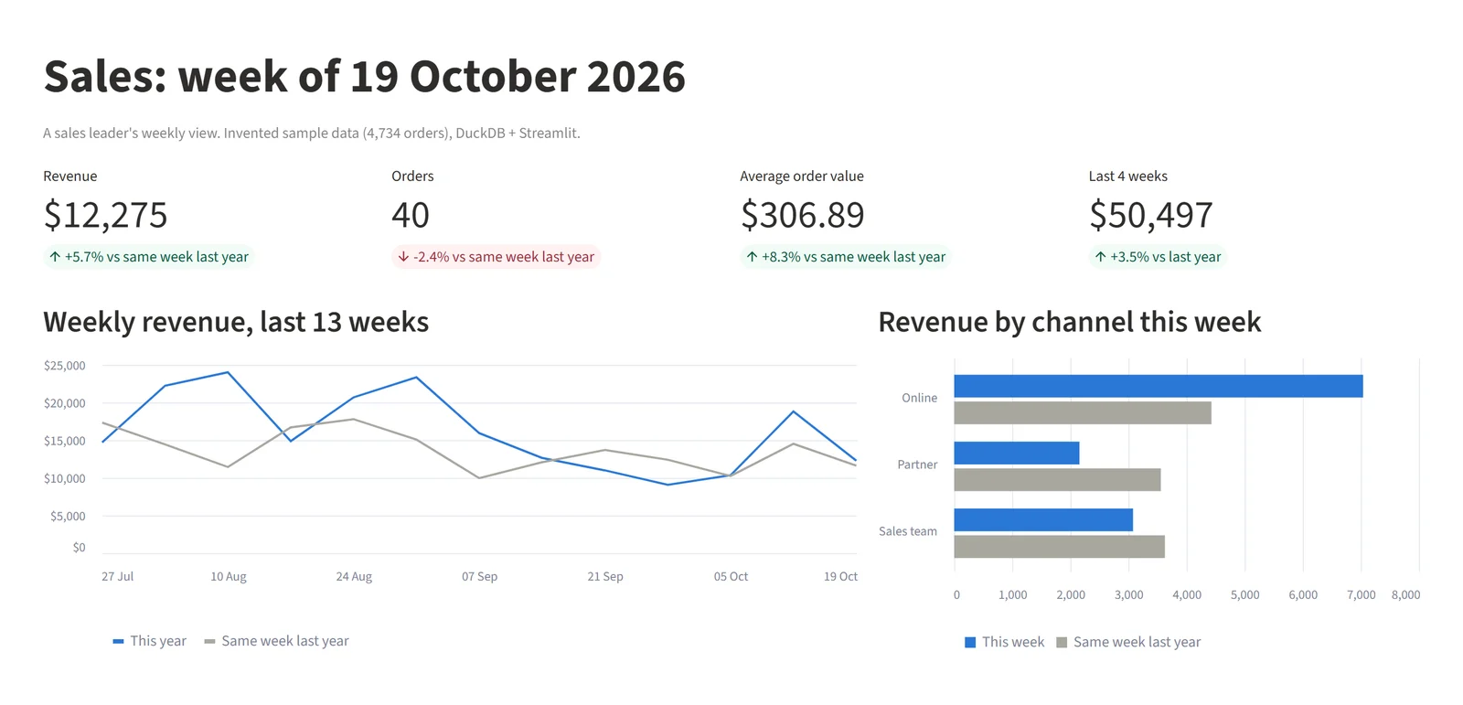
A sales leader's weekly view, a small Streamlit 1.67.0 app on DuckDB. Invented data.
2. A rep's territory and pipeline
A rep wants to know whether they will make their number. On it: their closed revenue against last year, open pipeline, win rate, pipeline coverage and deals closing this month. Salesforce defines win rate as "(Won Opportunities / Total Opportunities) x 100", and gives pipeline coverage as annual quota ÷ win rate ÷ (365 ÷ sales cycle in days): at a 25% win rate and a 60-day cycle, a $100,000 quota needs $65,757 in pipeline.
The sample has orders, not deals, so the query covers the closed half: the Sales team channel by region, standing in for territories. On your own data, group by the deal owner instead.
SELECT region AS territory,
       count(*) FILTER (WHERE year(order_date) = 2026)          AS orders_q3_2026,
       round(sum(revenue) FILTER (WHERE year(order_date) = 2026)) AS q3_2026,
       round(sum(revenue) FILTER (WHERE year(order_date) = 2025)) AS q3_2025,
       round(100 * (sum(revenue) FILTER (WHERE year(order_date) = 2026)
                  / sum(revenue) FILTER (WHERE year(order_date) = 2025) - 1), 1) AS change_pct
FROM sales
WHERE channel = 'Sales team'
  AND quarter(order_date) = 3
GROUP BY region
ORDER BY q3_2026 DESC;
┌───────────┬────────────────┬─────────┬─────────┬────────────┐
│ territory │ orders_q3_2026 │ q3_2026 │ q3_2025 │ change_pct │
│ varchar │ int64 │ double │ double │ double │
├───────────┼────────────────┼─────────┼─────────┼────────────┤
│ West │ 81 │ 26432.0 │ 15563.0 │ 69.8 │
│ North │ 58 │ 19014.0 │ 15532.0 │ 22.4 │
│ East │ 55 │ 16664.0 │ 14806.0 │ 12.5 │
│ South │ 41 │ 9667.0 │ 10627.0 │ -9.0 │
└───────────┴────────────────┴─────────┴─────────┴────────────┘South is the only territory that shrank, and it is $960 behind: at its $236 average order, about four orders. Put the order count beside each number, so nobody reads a small sample as a trend.
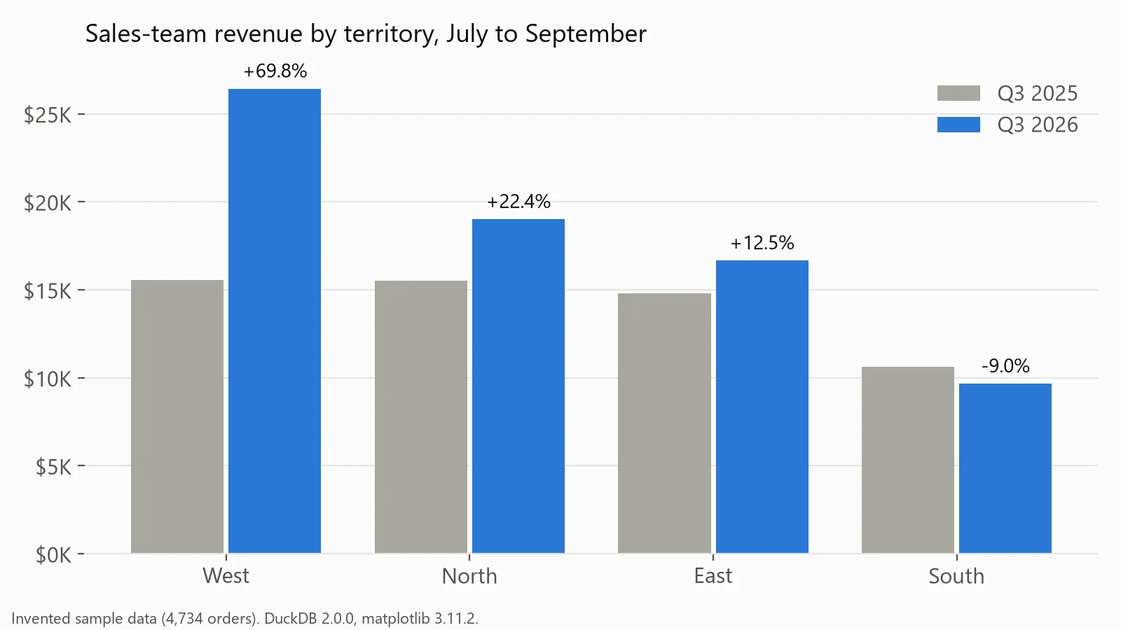
Sales-team revenue by territory, Q3 2026 against Q3 2025. Drawn in matplotlib from invented data.
3. A regional view
Regional managers want to know whose region is growing and whose is just big. On it: revenue, share of the total and growth for each region, over 12 months so the season cancels out.
SELECT region,
       round(sum(revenue) FILTER (WHERE order_date >= DATE '2025-11-01')) AS last_12m,
       round(100 * sum(revenue) FILTER (WHERE order_date >= DATE '2025-11-01')
             / sum(sum(revenue) FILTER (WHERE order_date >= DATE '2025-11-01')) OVER (), 1) AS share_pct,
       round(100 * (sum(revenue) FILTER (WHERE order_date >= DATE '2025-11-01')
                  / sum(revenue) FILTER (WHERE order_date <  DATE '2025-11-01') - 1), 1) AS yoy_pct
FROM sales
GROUP BY region
ORDER BY last_12m DESC;
┌─────────┬──────────┬───────────┬─────────┐
│ region │ last_12m │ share_pct │ yoy_pct │
│ varchar │ double │ double │ double │
├─────────┼──────────┼───────────┼─────────┤
│ West │ 233008.0 │ 28.5 │ 29.1 │
│ North │ 226995.0 │ 27.8 │ 19.2 │
│ East │ 185228.0 │ 22.7 │ 22.7 │
│ South │ 171499.0 │ 21.0 │ 27.0 │
└─────────┴──────────┴───────────┴─────────┘South is the smallest region but the second fastest-growing, which a chart sorted by revenue alone hides. With many regions or countries, use horizontal bars so the names fit (types of charts has the rules).
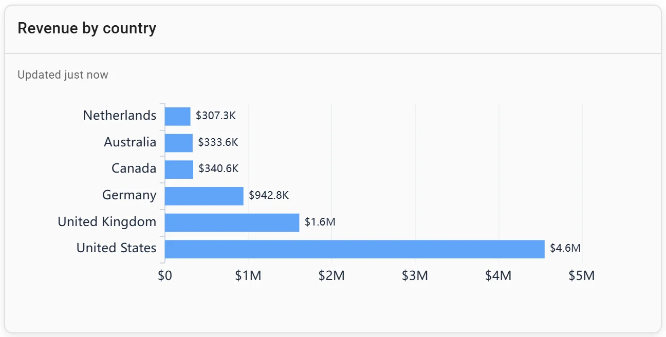
A horizontal bar chart: revenue by country. Invented data.
4. A channel view
Whoever runs partners or sales operations wants to know whether the mix is shifting. On it: revenue by channel each quarter, as amounts and as shares.
SELECT year(order_date) || '-Q' || quarter(order_date) AS quarter,
       round(sum(revenue))                                                       AS revenue,
       round(100 * sum(revenue) FILTER (WHERE channel = 'Online')     / sum(revenue), 1) AS online_pct,
       round(100 * sum(revenue) FILTER (WHERE channel = 'Sales team') / sum(revenue), 1) AS sales_team_pct,
       round(100 * sum(revenue) FILTER (WHERE channel = 'Partner')    / sum(revenue), 1) AS partner_pct
FROM sales
WHERE order_date >= DATE '2025-10-01' AND order_date < DATE '2026-10-01'   -- last 4 full quarters
GROUP BY 1
ORDER BY 1;
┌─────────┬──────────┬────────────┬────────────────┬─────────────┐
│ quarter │ revenue │ online_pct │ sales_team_pct │ partner_pct │
│ varchar │ double │ double │ double │ double │
├─────────┼──────────┼────────────┼────────────────┼─────────────┤
│ 2025-Q4 │ 177800.0 │ 47.1 │ 32.5 │ 20.4 │
│ 2026-Q1 │ 171169.0 │ 47.9 │ 27.0 │ 25.1 │
│ 2026-Q2 │ 227206.0 │ 50.3 │ 29.3 │ 20.4 │
│ 2026-Q3 │ 236159.0 │ 49.0 │ 30.4 │ 20.7 │
└─────────┴──────────┴────────────┴────────────────┴─────────────┘The mix barely moved: partners peaked at 25.1% in the first quarter of 2026 and fell back. A stacked bar shows the total and its split at once.
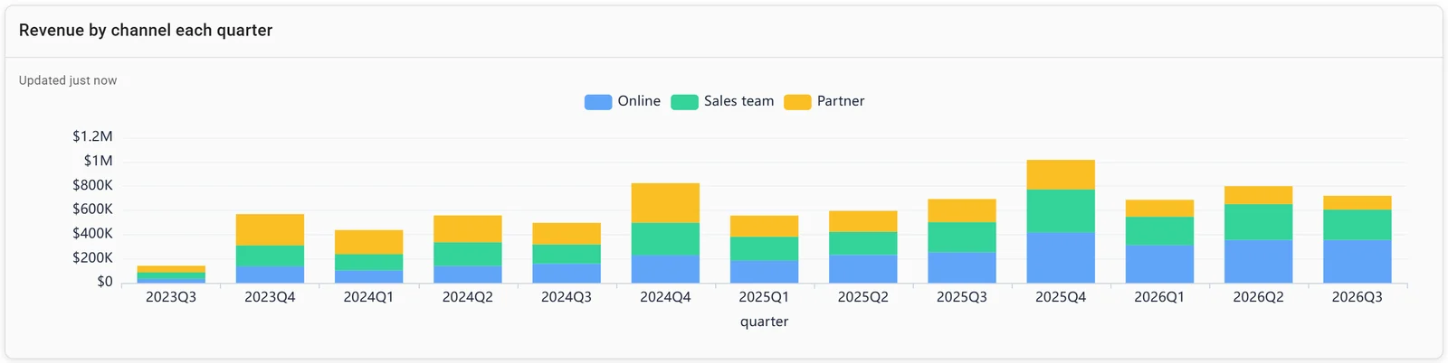
A stacked bar chart: revenue by channel each quarter. Invented data.
5. A product mix view
Product and category leads want to know what sells and what's fading. On it: the top products by revenue, each with its share and growth, plus a treemap for the long tail.
SELECT product,
       round(sum(revenue) FILTER (WHERE order_date >= DATE '2025-11-01')) AS last_12m,
       round(100 * sum(revenue) FILTER (WHERE order_date >= DATE '2025-11-01')
             / sum(sum(revenue) FILTER (WHERE order_date >= DATE '2025-11-01')) OVER (), 1) AS share_pct,
       round(100 * (sum(revenue) FILTER (WHERE order_date >= DATE '2025-11-01')
                  / sum(revenue) FILTER (WHERE order_date <  DATE '2025-11-01') - 1), 1) AS yoy_pct
FROM sales
GROUP BY product
ORDER BY last_12m DESC
LIMIT 5;
┌──────────────────┬──────────┬───────────┬─────────┐
│ product │ last_12m │ share_pct │ yoy_pct │
│ varchar │ double │ double │ double │
├──────────────────┼──────────┼───────────┼─────────┤
│ Standing desk │ 221174.0 │ 27.1 │ 48.4 │
│ Office chair │ 116849.0 │ 14.3 │ 21.3 │
│ Team plan │ 109105.0 │ 13.4 │ 17.2 │
│ Training day │ 54894.0 │ 6.7 │ -7.1 │
│ Reporting add-on │ 54304.0 │ 6.6 │ 6.8 │
└──────────────────┴──────────┴───────────┴─────────┘One product of 13 brings in 27.1% of revenue and grew 48.4%: worth a tile of its own. Training day is the only top-five product in decline.
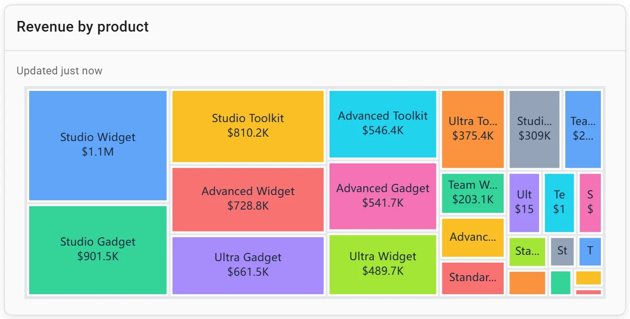
A treemap: revenue by product. Invented data.
Connect any database. Ask in plain English.
Start free →6. A customer segment view
Account managers want to know who buys and how much each order is worth. On it: orders, share of revenue, average order value and units per order for each segment.
SELECT segment,
       count(*)                                                  AS orders,
       round(100 * sum(revenue) / sum(sum(revenue)) OVER (), 1)  AS share_pct,
       round(sum(revenue) / count(*), 2)                         AS avg_order_value,
       round(sum(quantity) / count(*), 2)                        AS units_per_order
FROM sales
WHERE order_date >= DATE '2025-11-01'      -- the last 12 months
GROUP BY segment
ORDER BY share_pct DESC;
┌────────────────┬────────┬───────────┬─────────────────┬─────────────────┐
│ segment │ orders │ share_pct │ avg_order_value │ units_per_order │
│ varchar │ int64 │ double │ double │ double │
├────────────────┼────────┼───────────┼─────────────────┼─────────────────┤
│ Small business │ 1434 │ 56.8 │ 323.42 │ 3.76 │
│ Mid-market │ 859 │ 30.2 │ 287.36 │ 3.69 │
│ Enterprise │ 335 │ 13.0 │ 316.72 │ 3.84 │
└────────────────┴────────┴───────────┴─────────────────┴─────────────────┘In this invented data, enterprise orders are no bigger than small-business ones, so the segments differ in volume only. On real data, that order-value column is what tells you whether chasing larger accounts pays. With a customer id, plot one bubble per customer.
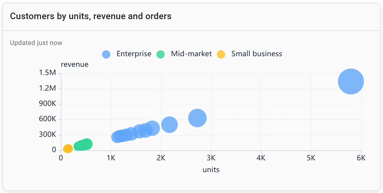
A bubble chart: customers by units, revenue and orders. Invented data.
7. A seasonality view
Sales ops needs the busy months before setting targets and hiring. On it: each month's revenue against the average month of its year, for two years, and orders by month and category.
WITH m AS (
  SELECT date_trunc('month', order_date) AS month,
         order_date >= DATE '2025-11-01'  AS year_2,      -- Nov 2025 to Oct 2026
         sum(revenue)                    AS revenue
  FROM sales
  GROUP BY ALL
),
idx AS (   -- each month against the average month of its own 12
  SELECT month, year_2, 100 * revenue / avg(revenue) OVER (PARTITION BY year_2) AS idx
  FROM m
)
SELECT strftime(month, '%b')               AS month,
       round(max(idx) FILTER (WHERE NOT year_2)) AS year_1_index,
       round(max(idx) FILTER (WHERE year_2))     AS year_2_index
FROM idx
GROUP BY 1
ORDER BY year_2_index DESC
LIMIT 4;
┌─────────┬──────────────┬──────────────┐
│ month │ year_1_index │ year_2_index │
│ varchar │ double │ double │
├─────────┼──────────────┼──────────────┤
│ Aug │ 124.0 │ 128.0 │
│ Jul │ 112.0 │ 124.0 │
│ Jun │ 135.0 │ 116.0 │
│ May │ 118.0 │ 112.0 │
└─────────┴──────────────┴──────────────┘The same four months, May to August, are the busiest in both years, 12% to 35% above an average month. A monthly target spread evenly will look missed all winter and beaten all summer.
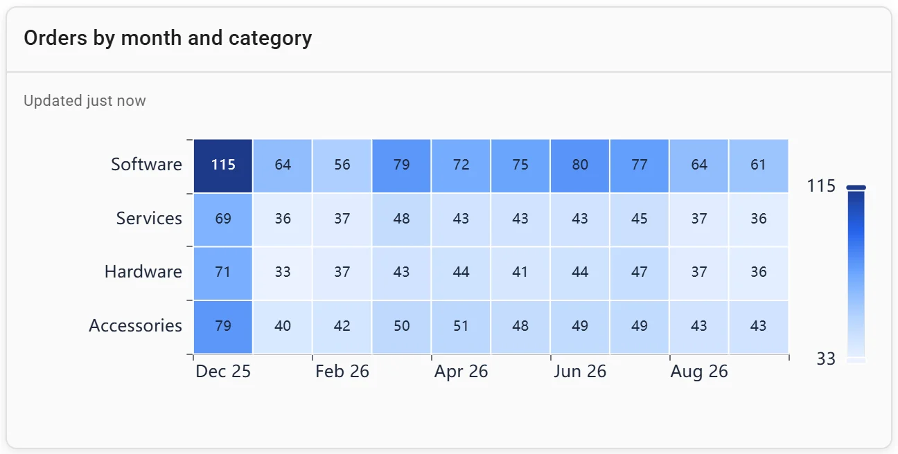
A heatmap: orders by month and category. Invented data.
8. A month-to-date pace view
Mid-month, the sales manager wants to know where the month will land. On it: revenue so far, a projection, and last year's same month. We stopped October at day 15 and projected it two ways:
WITH oct AS (
  SELECT year(order_date)                                   AS year,
         sum(revenue) FILTER (WHERE day(order_date) <= 15)  AS first_15_days,
         sum(revenue)                                       AS actual_month
  FROM sales
  WHERE month(order_date) = 10
  GROUP BY 1
)
SELECT year,
       round(first_15_days)                 AS first_15_days,
       round(first_15_days * 31 / 15)       AS straight_line,
       round(first_15_days / (lag(first_15_days) OVER w / lag(actual_month) OVER w)) AS last_years_shape,
       round(actual_month)                  AS actual_month
FROM oct
WINDOW w AS (ORDER BY year)
ORDER BY year;
┌───────┬───────────────┬───────────────┬──────────────────┬──────────────┐
│ year │ first_15_days │ straight_line │ last_years_shape │ actual_month │
│ int64 │ double │ double │ double │ double │
├───────┼───────────────┼───────────────┼──────────────────┼──────────────┤
│ 2025 │ 23223.0 │ 47995.0 │ NULL │ 53122.0 │
│ 2026 │ 23508.0 │ 48584.0 │ 53773.0 │ 57518.0 │
└───────┴───────────────┴───────────────┴──────────────────┴──────────────┘A straight line said October 2026 would finish at $48,584; it closed at $57,518, 18.4% higher, because the second half of October is busier in both years (in 2026, $2,126 a day after the 15th against $1,567 before). Scaling by last year's first-half share gave $53,773, closer. Show the projection with last year's line beside it, not alone.
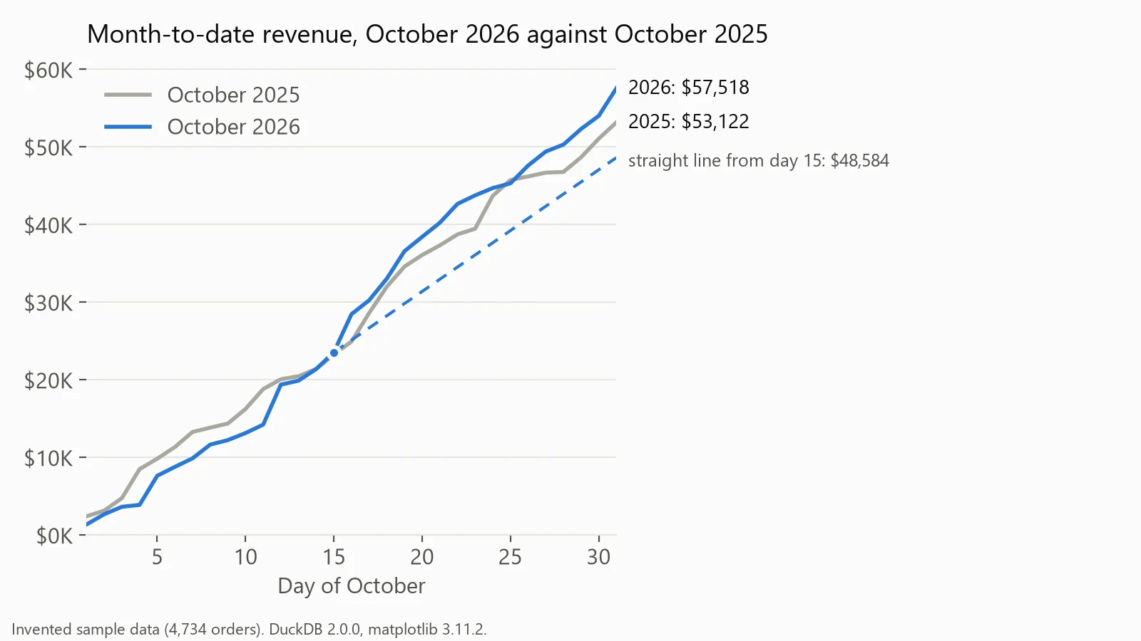
Month-to-date revenue for October, with a straight-line projection from day 15. Drawn in matplotlib from invented data.
9. A founder's month-end revenue view
At month-end, the founder wants one answer: did revenue grow, and which part of the business did it? On it: the month against the same month last year, the year so far, and a bridge from last year's month to this one by category.
SELECT coalesce(category, 'Total') AS category,
       round(sum(revenue) FILTER (WHERE year(order_date) = 2025)) AS oct_2025,
       round(sum(revenue) FILTER (WHERE year(order_date) = 2026)) AS oct_2026,
       round(sum(revenue) FILTER (WHERE year(order_date) = 2026)
           - sum(revenue) FILTER (WHERE year(order_date) = 2025)) AS change
FROM sales
WHERE month(order_date) = 10
GROUP BY ROLLUP (category)
ORDER BY grouping(category), change DESC;
┌──────────┬──────────┬──────────┬─────────┐
│ category │ oct_2025 │ oct_2026 │ change │
│ varchar │ double │ double │ double │
├──────────┼──────────┼──────────┼─────────┤
│ Software │ 13088.0 │ 17524.0 │ 4436.0 │
│ Supplies │ 7587.0 │ 9735.0 │ 2148.0 │
│ Services │ 7272.0 │ 8134.0 │ 862.0 │
│ Hardware │ 25175.0 │ 22125.0 │ -3050.0 │
│ Total │ 53122.0 │ 57518.0 │ 4396.0 │
└──────────┴──────────┴──────────┴─────────┘October grew $4,396, and Software alone added more than that, while Hardware, the biggest category and the fastest-growing over 12 months in our KPI examples, fell $3,050. That is the bridge's job: a total that hides a falling core. Draw it as a waterfall (revenue waterfall in SQL). For the same numbers as a written note, see our weekly report template.
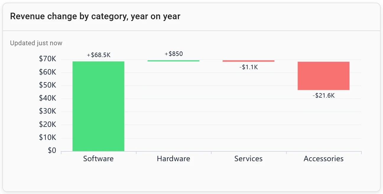
A waterfall chart: revenue change by category, year on year. Invented data.
Building a sales dashboard for a team or a client
Each example above is a few saved queries. Fastero is an AI and data platform where people and AI agents work together on a team's data:
- Connect once. Postgres, MySQL, SQL Server, Redshift, Oracle or BigQuery, or a CSV or Excel export from the CRM. Ask Fastero's assistant for any view above; every chart stays a saved query you can open and check.
- Viewers are free. The sales team signs in with its own logins. The Free plan is $0 with no end date; Pro is $20 per editor a month (checked 20 November 2026).
- Monday's email. A dashboard can email itself daily, weekly or monthly, with the numbers, charts and tables plus a PDF. People in the workspace also get a button that opens it in Fastero; anyone else gets the email and the PDF, and an address outside the workspace confirms first. The same dialog can post to Slack once Slack is connected.
- For a client. The Send dialog's "Just this person" sends one dashboard to an email address, and they see only that dashboard after a code sent to their inbox. "Anyone with the link" makes a public link you can turn off.
- Refresh. On a timer (1, 5, 15 or 60 minutes) or, for Postgres and BigQuery data only, when the data changes.
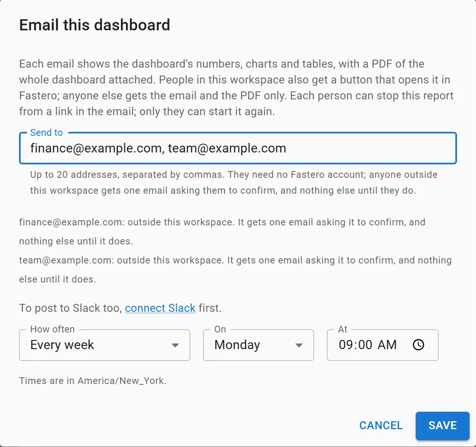
Setting up a weekly email of a dashboard, with invented addresses.
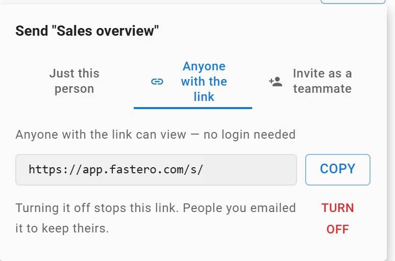
A dashboard's public link: anyone with it can view without a login, and turning it off stops it. Link shortened.
For what goes in a client's monthly report, see the client report template; for a leadership screen, executive dashboard examples.
FAQ
What should be on a sales dashboard?
Three to six numbers its reader acts on, each beside a comparison such as last year or a target, then one trend chart and one breakdown. For a head of sales that is revenue, orders and average order value against the same week last year, with revenue by channel.
What KPIs should a sales dashboard track?
Revenue, order or deal count and average order value for everyone; win rate, pipeline coverage and days to close for a team that sells through deals. Salesforce defines win rate as won opportunities divided by all opportunities, times 100.
What is the difference between a sales dashboard and a sales report?
A dashboard is a screen that stays current and is read often, for spotting what changed. A report is a fixed set of numbers for a period, usually sent with a written explanation. A dashboard emailed on a schedule does both jobs.
How do I make a sales dashboard?
Pick the reader and their question, write one query per number, compare each with the same period last year, and lay out the headline numbers first, then a trend, then a breakdown. Use full periods only, and keep the queries saved so every chart can be checked.
How often should a sales dashboard update?
As often as someone acts on it: daily for most sales views, more often for a rep working today's deals. A weekly leadership view can email itself before the Monday meeting.
What is a sales pipeline dashboard?
A view of open deals by stage, their value, expected close dates and the win rate that turns pipeline into revenue. Salesforce's coverage formula, quota ÷ win rate ÷ (365 ÷ sales cycle in days), says how much pipeline a rep needs.
Sources
Read on 20 November 2026:
- Salesforce: What is sales win rate, Why the 3x pipeline coverage rule is broken
- Queries: DuckDB 2.0.0 on Python 3.14.3, on an invented file of 4,734 orders, run 20 November 2026
- The weekly view: Streamlit 1.67.0 and Altair 6.3.0 on DuckDB 2.0.0; the other two charts drawn with matplotlib 3.11.2
Try Fastero free: connect your sales data, ask for the view your team needs, and send it every Monday. No credit card required.