 Fastero Dev Team
Plotly draws interactive charts from Python: hover for values, zoom, toggle series, and save as HTML or an image. Its documentation has a page per chart type; what's hard to find is one page of the common examples, run on the current version, with the chart each one draws. That's this page.
The short answer: install with pip install plotly, and use Plotly Express (import plotly.express as px) for nearly everything: px.line, px.bar, px.scatter, px.histogram, px.imshow, px.choropleth, px.treemap. Drop to plotly.graph_objects for two y-axes and mixed subplots. Plotly and Dash are both free and MIT-licensed. Every example below ran on Plotly 7.1.0, released 15 September 2026, with Python 3.14, using Plotly's bundled sample data or numbers we made up. Plotly 7 broke some old snippets: Mapbox maps, create_distplot and the other figure-factory helpers, engine= in write_image, and titlefont= all fail now.
Fastero
Run a Streamlit dashboard like these on your own data.
Every new Fastero workspace starts with a sample Streamlit app you can run and edit. Deploy your own from GitHub with your team's login and secrets built in: no Docker, no auth proxy.
Try free →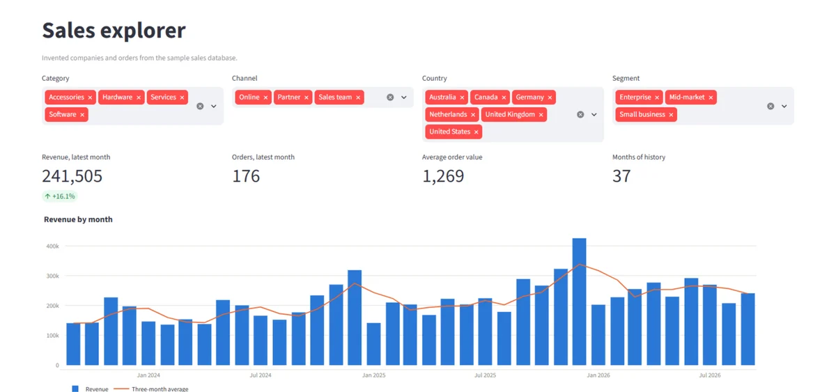
Setup
pip install plotly pandas          # charts
pip install kaleido                # to save PNG, SVG or PDF; needs Google Chrome installed
pip install dash                   # for the Dash app at the end
Every example ends with fig.write_image(...) to save the picture shown; in a notebook, fig.show() or just fig on the last line displays it interactively instead. We saved at width=800, height=450, scale=2: an 800-pixel layout at double density, which keeps labels readable once a page shrinks the image.
1. Line chart: several series
import plotly.express as px

df = px.data.stocks()  # weekly closing prices, each rebased to 1.0 on 2018-01-01

fig = px.line(
    df,
    x="date",
    y=["GOOG", "AAPL", "AMZN", "MSFT"],  # a list of columns = one line per column
    title="Four stocks, rebased to 1.0 on 1 January 2018",
    labels={"value": "Price (1.0 = start)", "variable": "Ticker", "date": ""},
)
fig.write_image("line.png", width=800, height=450, scale=2)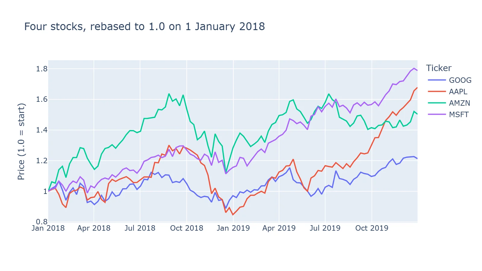
Passing a list of columns as y draws one line per column from wide data. For long data (one row per date and series), pass the series column as color= instead.
2. Grouped bar chart
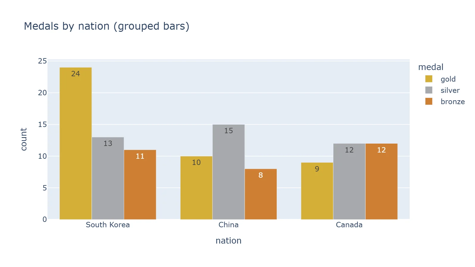
df = px.data.medals_long()  # columns: nation, medal, count

fig = px.bar(
    df,
    x="nation",
    y="count",
    color="medal",
    barmode="group",  # side by side; the default is stacked
    text_auto=True,
    color_discrete_map={"gold": "#D4AF37", "silver": "#A8A9AD", "bronze": "#CD7F32"},
    title="Medals by nation (grouped bars)",
)
3. Stacked bar chart
df = px.data.tips()
# Aggregate first: px.bar on raw rows draws one thin segment per row.
totals = df.groupby(["day", "time"], as_index=False)["total_bill"].sum()

fig = px.bar(
    totals,
    x="day",
    y="total_bill",
    color="time",
    barmode="stack",
    text_auto=".0f",
    category_orders={"day": ["Thur", "Fri", "Sat", "Sun"]},
    labels={"total_bill": "Total bills ($)", "day": "", "time": ""},
    title="Takings by day, lunch vs dinner (stacked bars)",
)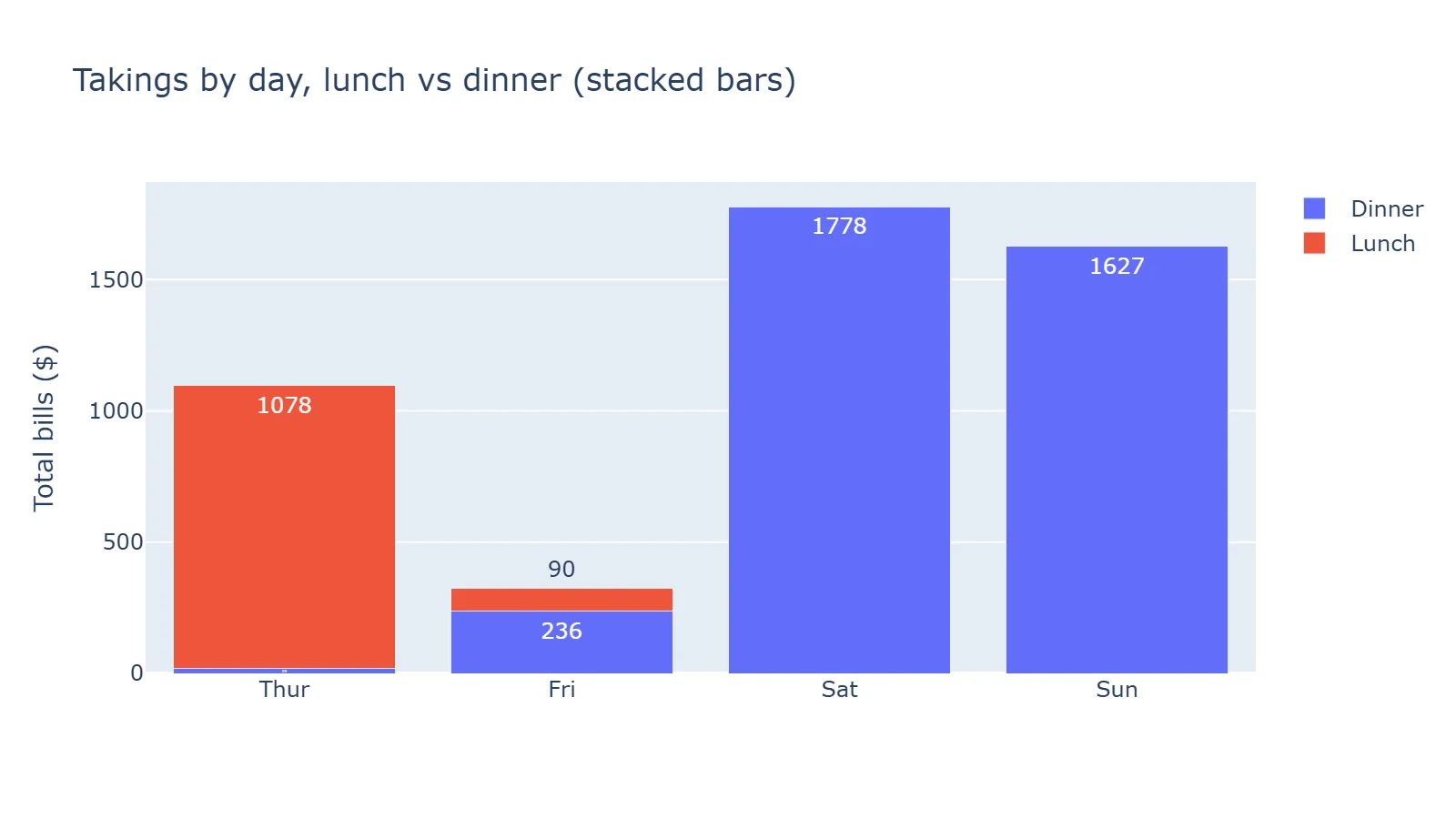
Two habits from this one. Sum the data before px.bar, or each row becomes its own thin slice of the bar. And set category_orders, or the days come out alphabetically.
4. Bubble chart with a hover tooltip
df = px.data.gapminder().query("year == 2007")

fig = px.scatter(
    df,
    x="gdpPercap",
    y="lifeExp",
    size="pop",
    color="continent",
    hover_name="country",
    hover_data={"pop": ":,", "gdpPercap": ":$,.0f"},  # format strings for the tooltip
    log_x=True,
    size_max=60,
    labels={"gdpPercap": "GDP per capita (log scale)", "lifeExp": "Life expectancy (years)"},
    title="GDP per capita vs life expectancy, 2007",
)
fig.write_html("bubble.html", include_plotlyjs="cdn")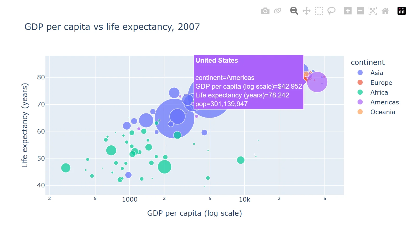
hover_name puts the country in bold at the top of the tooltip; hover_data formats the other values. This is the screenshot of the HTML file in a browser, the way readers meet a Plotly chart.
5. Histogram with box plots
df = px.data.tips()

fig = px.histogram(
    df,
    x="total_bill",
    color="sex",
    nbins=30,
    barmode="overlay",
    opacity=0.65,
    marginal="box",  # adds a box plot above the histogram
    labels={"total_bill": "Bill total ($)"},
    title="Distribution of bill totals",
)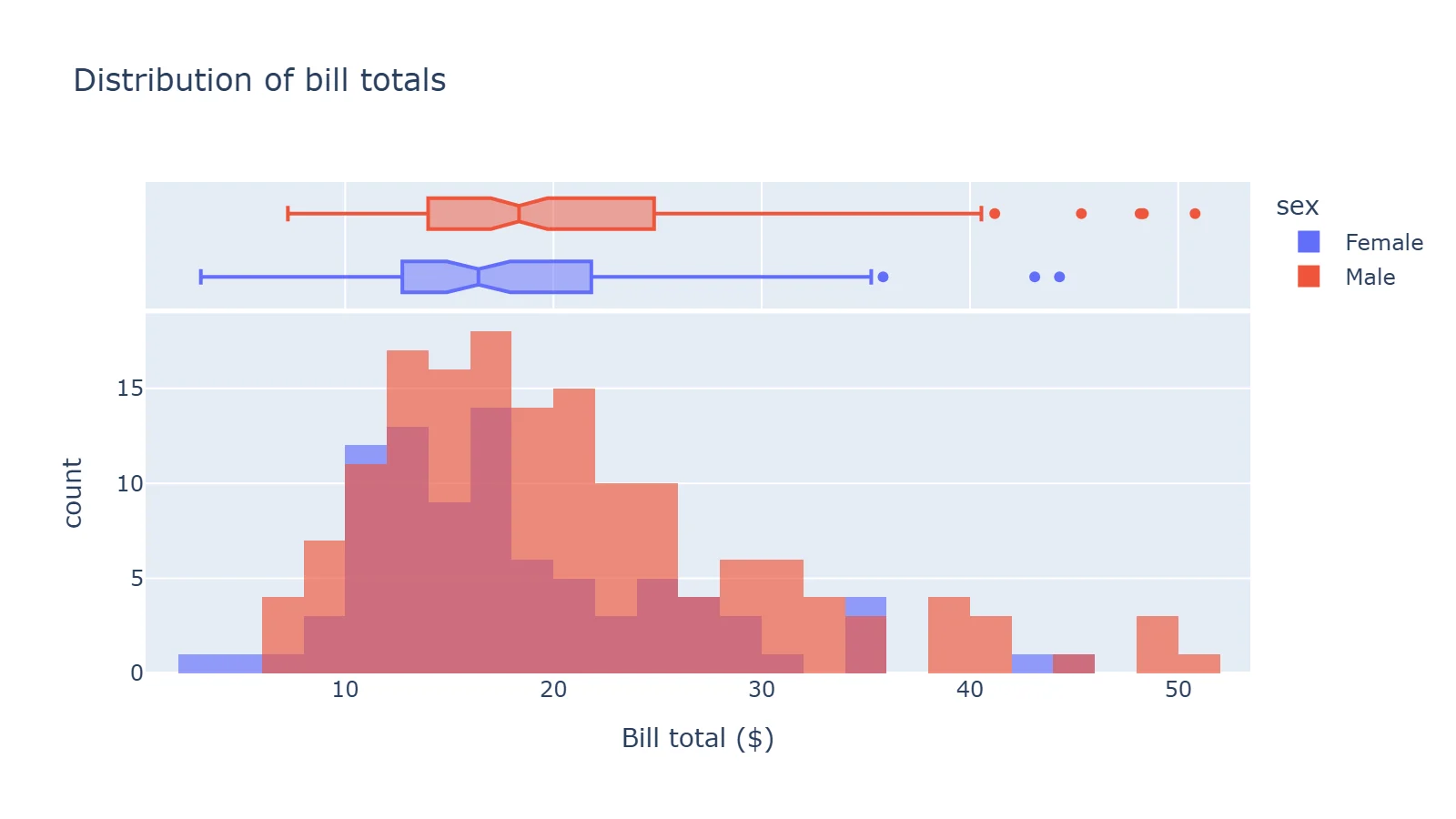
marginal also takes "violin", "rug" or "histogram". For a violin or box plot on its own, px.violin and px.box take the same x, y and color arguments.
6. Correlation heatmap
df = px.data.iris()
corr = df[["sepal_length", "sepal_width", "petal_length", "petal_width"]].corr()

fig = px.imshow(
    corr,
    text_auto=".2f",               # print the value in each cell
    color_continuous_scale="RdBu_r",
    zmin=-1,
    zmax=1,
    title="Correlation between iris measurements",
)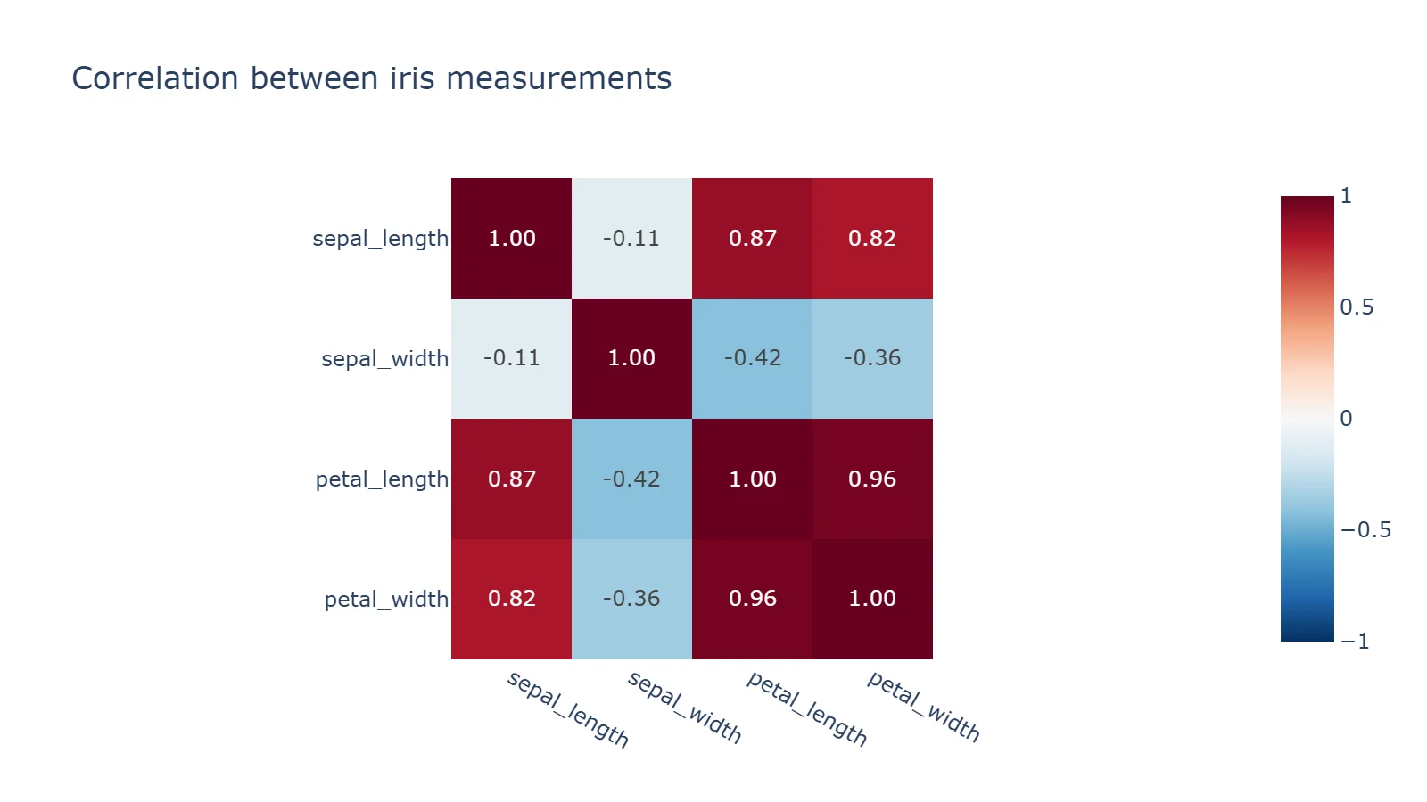
px.imshow with text_auto replaces ff.create_annotated_heatmap, which no longer exists in Plotly 7. Pin zmin and zmax to -1 and 1 so the colour scale is centred on zero.
7. Donut chart
df = px.data.tips()

# Rows with the same name are summed into one slice.
fig = px.pie(df, values="tip", names="day", hole=0.45, title="Share of tips by day")
fig.update_traces(textposition="inside", textinfo="percent+label")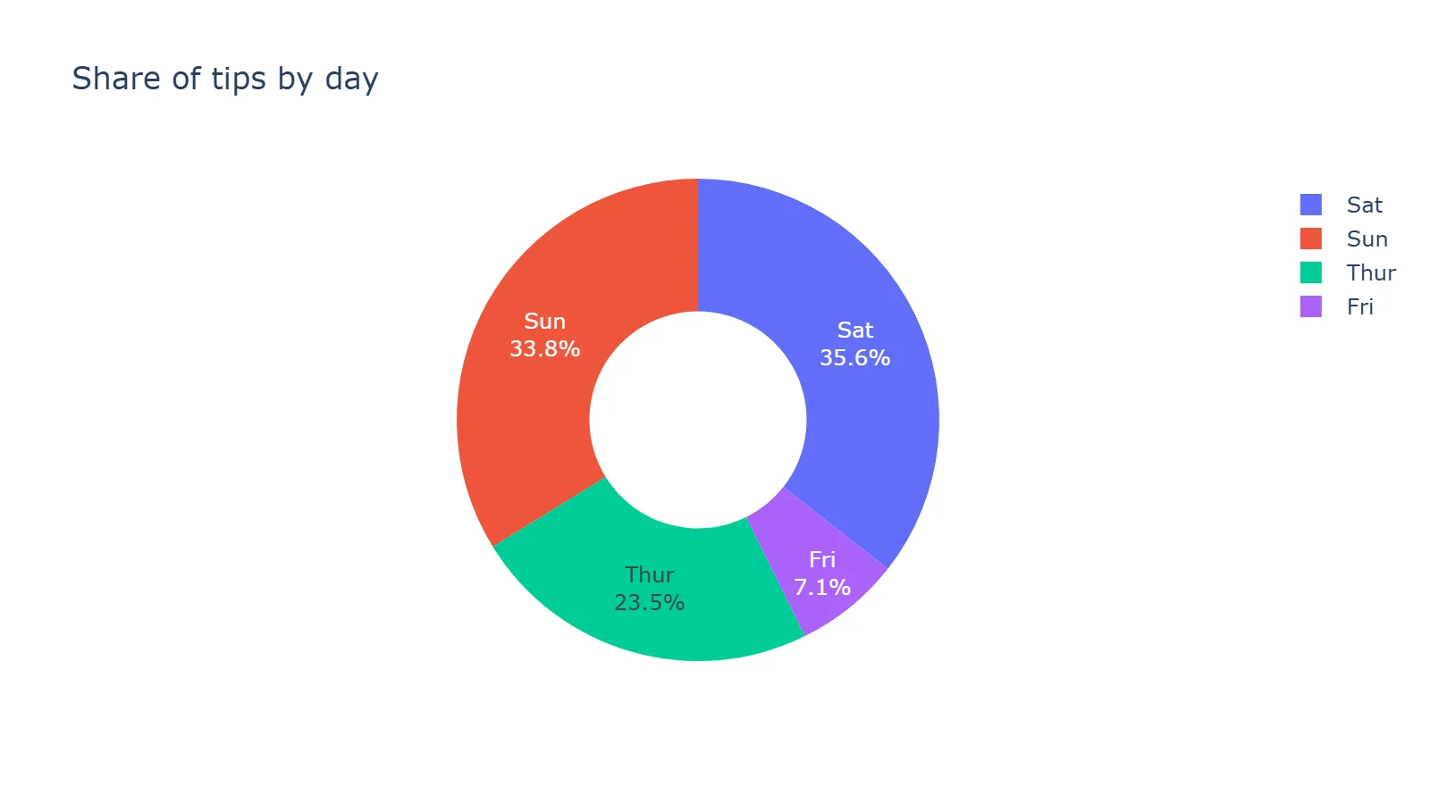
8. World map (choropleth)
df = px.data.gapminder().query("year == 2007")

fig = px.choropleth(
    df,
    locations="iso_alpha",  # ISO-3 country codes
    color="lifeExp",
    hover_name="country",
    color_continuous_scale="Viridis",
    projection="natural earth",
    labels={"lifeExp": "Life exp."},
    title="Life expectancy by country, 2007",
)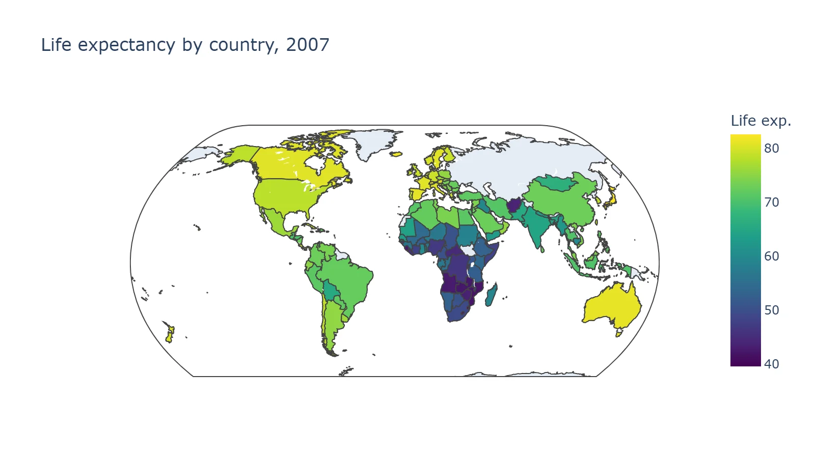
Countries missing from the data stay grey, as Russia and Greenland do here. In Plotly 7, maps "now fit their initial view to the locations they plot"; pass fitbounds=False to get the old full-world view.
9. Treemap
df = px.data.gapminder().query("year == 2007")

fig = px.treemap(
    df,
    path=[px.Constant("World"), "continent", "country"],  # outer level -> inner level
    values="pop",
    color="lifeExp",
    color_continuous_scale="RdYlGn",
    labels={"lifeExp": "Life exp."},
    title="Population by continent and country, coloured by life expectancy (2007)",
)
fig.update_layout(margin=dict(t=50, l=10, r=10, b=10))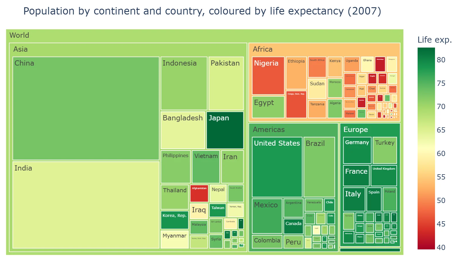
10. Funnel
import pandas as pd

# Invented numbers for an online shop
df = pd.DataFrame({
    "stage": ["Visited site", "Viewed a product", "Added to cart", "Started checkout", "Purchased"],
    "visitors": [10000, 6200, 2300, 1100, 870],
})

fig = px.funnel(df, x="visitors", y="stage", labels={"stage": ""}, title="Checkout funnel (invented data)")
fig.update_traces(texttemplate="%{value:,}<br>%{percentInitial:.0%} of visitors")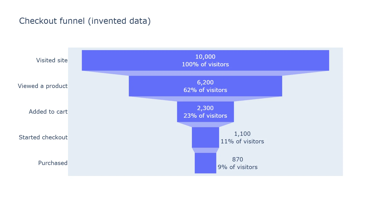
%{percentInitial} is each stage's share of the first one; %{percentPrevious} gives step-to-step conversion instead.
11. Several charts in one figure
import plotly.graph_objects as go
from plotly.subplots import make_subplots

stocks = px.data.stocks()
tips = px.data.tips()
days = ["Thur", "Fri", "Sat", "Sun"]
by_day = tips.groupby("day")["total_bill"].sum().reindex(days)  # groupby sorts days A-Z

fig = make_subplots(rows=2, cols=2,
                    subplot_titles=("GOOG price", "Takings by day", "Tip distribution", "Bill vs tip"))
fig.add_trace(go.Scatter(x=stocks["date"], y=stocks["GOOG"], mode="lines", name="GOOG"), row=1, col=1)
fig.add_trace(go.Bar(x=by_day.index, y=by_day.values, name="Takings", width=0.7), row=1, col=2)
fig.add_trace(go.Histogram(x=tips["tip"], nbinsx=20, name="Tips"), row=2, col=1)
fig.add_trace(go.Scatter(x=tips["total_bill"], y=tips["tip"], mode="markers", name="Bills"), row=2, col=2)
fig.update_layout(title="Four charts in one figure with make_subplots", showlegend=False)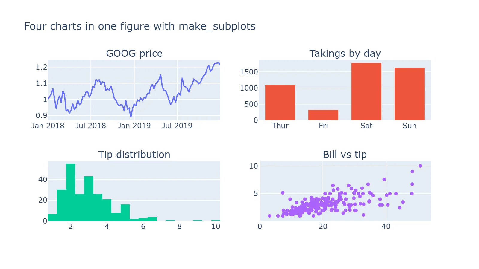
Note width=0.7 on the bars. Without it, the bars touch: a histogram anywhere in a figure sets the gap between bars to zero for the whole figure, bar charts included.
Run a Streamlit dashboard like these.
Start free →12. Two y-axes
import plotly.graph_objects as go
from plotly.subplots import make_subplots

# Invented monthly figures for a small shop
months = ["Jan", "Feb", "Mar", "Apr", "May", "Jun", "Jul", "Aug", "Sep", "Oct", "Nov", "Dec"]
orders = [420, 390, 510, 560, 610, 580, 640, 700, 660, 720, 910, 1180]
avg_order = [38.5, 37.9, 39.2, 40.1, 41.0, 40.4, 41.8, 42.5, 42.1, 43.0, 45.6, 48.9]

fig = make_subplots(specs=[[{"secondary_y": True}]])
fig.add_trace(go.Bar(x=months, y=orders, name="Orders"), secondary_y=False)
fig.add_trace(go.Scatter(x=months, y=avg_order, name="Average order ($)", mode="lines+markers"), secondary_y=True)
fig.add_hline(y=600, line_dash="dot", annotation_text="Target: 600 orders",
              annotation_position="top left", secondary_y=False)
# Plotly 7 lines the right axis's ticks up with the left axis's gridlines (tickmode="sync").
# Ranges that divide the same way (0-1200 and 0-60) give round numbers on both sides.
fig.update_yaxes(title_text="Orders", range=[0, 1200], secondary_y=False)
fig.update_yaxes(title_text="Average order", tickprefix="$", range=[0, 60], secondary_y=True)
fig.update_layout(title="Orders and average order value (invented data)", legend=dict(orientation="h", y=1.1))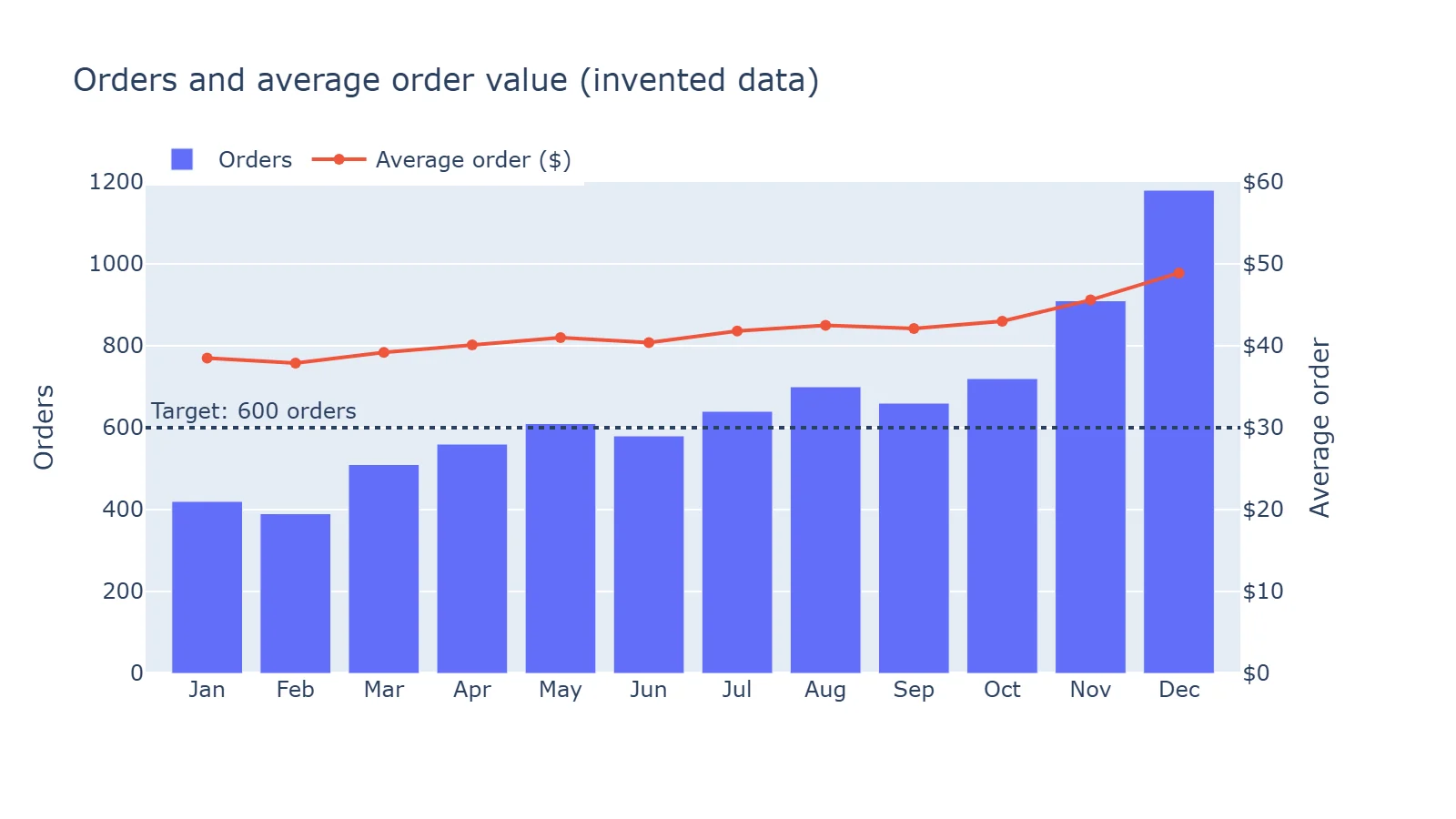
This one changed in Plotly 7. The right-hand axis now places its ticks on the left axis's gridlines, so without the two range= settings our first version labelled the right axis $37.09, $39.12, $41.16 and so on. Plotly's migration guide says tickmode="auto" on the right axis restores two independent grids. Use two axes sparingly, though: readers compare the heights of two unrelated scales, and two charts side by side are often clearer.
13. Animation
df = px.data.gapminder()

fig = px.scatter(
    df, x="gdpPercap", y="lifeExp", size="pop", color="continent", hover_name="country",
    animation_frame="year",     # one frame per year, with a slider and play button
    animation_group="country",  # tells Plotly which marker is which between frames
    log_x=True, size_max=55,
    range_x=[100, 100_000],     # fix the axes, or they rescale on every frame
    range_y=[25, 90],
    title="Gapminder, 1952-2007 (press play)",
)
fig.write_html("animation.html", auto_play=False)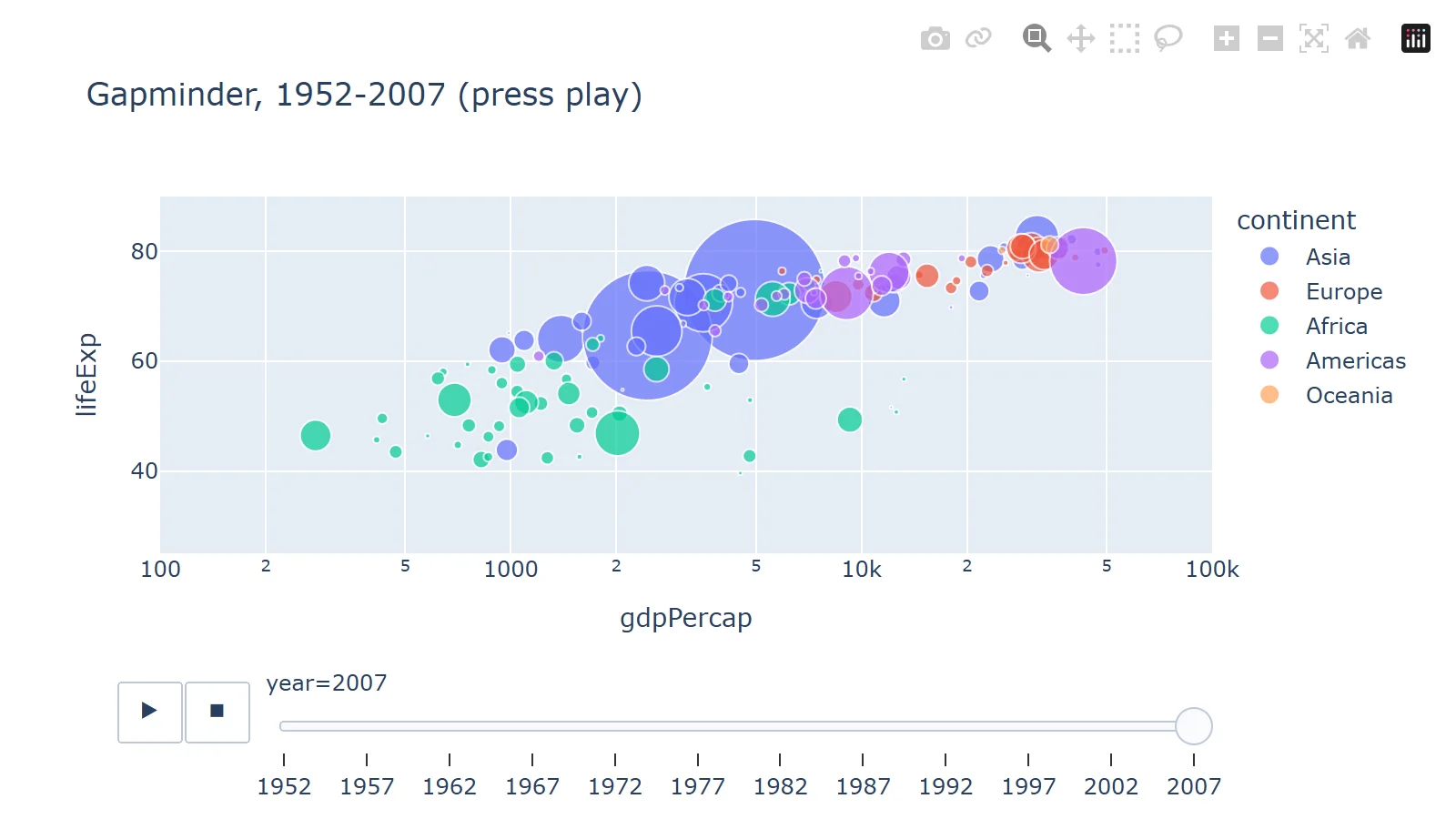
Fix both axis ranges, or the axes jump on every frame. A PNG of an animated figure shows only the first frame; animation needs the HTML.
14. A styled line chart
df = px.data.gapminder().query("country in ['Japan', 'Germany', 'Brazil', 'India', 'Nigeria']")

fig = px.line(df, x="year", y="gdpPercap", color="country", markers=True,
              template="plotly_white")  # also: simple_white, ggplot2, seaborn, plotly_dark, presentation
# With hovermode="x unified" Plotly adds the year and each line's name itself.
fig.update_traces(hovertemplate="<b>$%{y:,.0f}</b>")
fig.update_layout(
    title=dict(text="GDP per capita, 1952-2007", subtitle=dict(text="Gapminder data, US dollars")),
    yaxis=dict(title=None, tickprefix="$", tickformat=",.0f"),
    xaxis=dict(title=None, dtick=10),
    legend=dict(title=None, orientation="h", yanchor="top", y=-0.1, xanchor="left", x=0),
    hovermode="x unified",
    font=dict(size=13),
)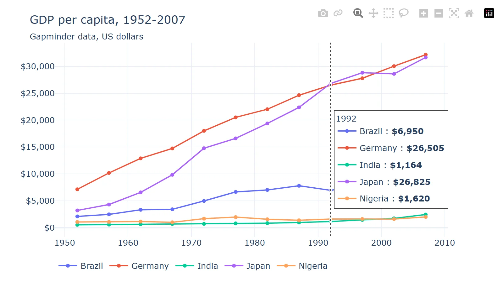
template sets the overall look, subtitle adds a second line under the title, and hovermode="x unified" shows every series' value at one x in a single tooltip. Our first try put a log scale on the y-axis with tickprefix="$"; the minor labels piled on top of each other and only $1,000 and $10,000 got the dollar sign, so we went back to a linear axis.
A Dash app with a dropdown
Dash turns Plotly charts into a web app, in Python. This one redraws the chart when you choose a continent:
from dash import Dash, Input, Output, callback, dcc, html
import plotly.express as px

df = px.data.gapminder()

app = Dash(__name__)
app.layout = html.Div(
    [
        html.H2("Life expectancy by country"),
        dcc.Dropdown(id="continent", options=sorted(df["continent"].unique()), value="Europe", clearable=False),
        dcc.Graph(id="chart", style={"height": "70vh"}),
    ],
    style={"maxWidth": "1100px", "margin": "0 auto", "fontFamily": "sans-serif"},
)


@callback(Output("chart", "figure"), Input("continent", "value"))
def update_chart(continent):
    subset = df[df["continent"] == continent]
    top = subset[subset["year"] == 2007].nlargest(8, "pop")["country"]  # 8 biggest countries
    return px.line(
        subset[subset["country"].isin(top)], x="year", y="lifeExp", color="country", markers=True,
        title=f"{continent}: the eight most populous countries",
        labels={"lifeExp": "Life expectancy (years)", "year": ""},
    )


if __name__ == "__main__":
    app.run(debug=True)  # http://127.0.0.1:8050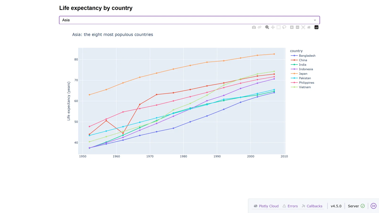
The @callback reads the dropdown's value and returns a new figure. Two things old tutorials get wrong: app.run_server() now fails with "app.run_server has been replaced by app.run", and import dash_core_components fails too; use from dash import dcc, html. The toolbar in the bottom corner appears because of debug=True.
Saving charts
fig.write_html("chart_full.html")                          # plotly.js embedded: opens offline
fig.write_html("chart_cdn.html", include_plotlyjs="cdn")   # loads plotly.js from cdn.plot.ly
fig.write_image("chart.png", width=800, height=450, scale=2)  # static files need kaleido + Chrome
fig.write_image("chart.svg")
fig.write_image("chart.pdf")| File | Size in our test |
|---|---|
chart_full.html |
4,831,434 bytes |
chart_cdn.html |
12,151 bytes |
chart.png |
103,209 bytes |
chart.svg |
38,853 bytes |
chart.pdf |
16,643 bytes |
A self-contained HTML file carries all of plotly.js, almost 5 MB; include_plotlyjs="cdn" cuts it to 12 KB but needs internet to open. For images, Kaleido 1.0 and later no longer bundle a browser: "Starting with Kaleido version 1.0.0, Chrome is not included in the package itself". If Chrome isn't installed, run plotly_get_chrome.
Each write_image starts and stops Chrome, which is slow in a loop. Saving five charts took 12 to 19 seconds that way, and 3 to 4.5 seconds after kaleido.start_sync_server(), which keeps one Chrome running for every call.
Blank charts in JupyterLab
If fig.show() runs and the output is empty, with no error, JupyterLab and Plotly are usually installed in different Python environments, as happens with JupyterHub or a conda base environment. Plotly's chart format needs its JupyterLab extension, which installs with Plotly, but only into the environment Plotly is in. We reproduced it: the cell ran and printed nothing. One line fixed it:
import plotly.io as pio
pio.renderers.default = "notebook"   # or fig.show(renderer="notebook")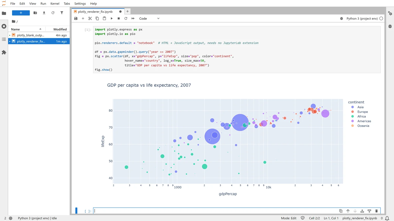
A kernel without nbformat raises "Mime type rendering requires nbformat>=4.2.0 but it is not installed"; pip install nbformat in the kernel's environment fixes that. VS Code and Colab are detected automatically.
What changed in Plotly 7
Plotly 7.0 arrived on 25 August 2026, with plotly.js 4. "Most figures render without any changes", but these old snippets now fail:
| Old code | What happens in Plotly 7 | Use instead |
|---|---|---|
px.scatter_mapbox, go.Scattermapbox |
AttributeError (Mapbox traces removed) |
px.scatter_map, go.Scattermap |
ff.create_distplot, ff.create_annotated_heatmap and other figure-factory helpers |
AttributeError |
px.histogram(..., marginal=...), px.imshow(..., text_auto=True) |
fig.write_image(..., engine="kaleido") |
TypeError: write_image() got an unexpected keyword argument 'engine' |
Drop engine; install Kaleido 1.x |
update_layout(titlefont=...) |
ValueError: Invalid property specified (removed in Plotly 6) |
title=dict(font=dict(...)) |
| Two y-axes | Right axis ticks now follow the left axis's grid | Set ranges, or tickmode="auto" |
| Maps | Initial view fits the plotted locations | fitbounds=False for the world view |
rgb(0.5, 0.5, 0.5) |
Now read as near black (CSS Color 4) | rgb(128, 128, 128) |
Sharing Plotly charts with a team
A Plotly chart in a notebook reaches the people who can run the notebook. To give colleagues a live page, wrap the charts in an app: Dash, or Streamlit, which displays a Plotly figure with st.plotly_chart(fig). Plotly sells hosting for Dash (Plotly Cloud, with a free tier and Pro at $29 per creator seat a month). Fastero hosts Streamlit apps behind your team's login, with Plotly already installed and database credentials kept in Secrets rather than in the code.
FAQ
Is Plotly free?
Yes. Plotly for Python and Dash are open source under the MIT licence. Plotly's paid products are Plotly Cloud, Plotly Studio and Dash Enterprise.
What's the difference between Plotly Express and graph_objects?
Plotly Express (px) builds a whole figure from a DataFrame in one call. It returns a graph_objects figure, which you use directly for things Express doesn't do, such as two y-axes or subplots mixing chart types.
How do I save a Plotly chart as a PNG?
pip install kaleido, make sure Google Chrome is installed (or run plotly_get_chrome), then fig.write_image("chart.png"). Add scale=2 for a sharper image.
Why is my Plotly chart blank in Jupyter?
Usually JupyterLab and Plotly are in different Python environments. Set pio.renderers.default = "notebook", or install Plotly in the environment JupyterLab runs from.
What is the latest version of Plotly?
Plotly 7.1.0, released 15 September 2026. Dash's latest is 4.5.0, from 29 October 2026.
How do I make an interactive Plotly chart I can send to someone?
fig.write_html("chart.html") makes one file that opens in any browser, with hover and zoom, and no Python needed.
Related reading:
Sources: plotly on PyPI, Dash on PyPI, Plotly 7 migration guide, Plotly 6 migration guide, plotly.py changelog, static image export, renderers, troubleshooting, Kaleido, Dash in Jupyter, is Plotly free?, Plotly Cloud pricing. Every example ran on 8 November 2026 with plotly 7.1.0, dash 4.5.0, kaleido 1.5.0 and pandas 3.1.1 on Python 3.14.
Try Fastero free — host Streamlit apps with Plotly charts behind your team's login, next to your databases. No credit card required.