Matplotlib Examples (2026): 10 Business Charts With Code You Can Copy

Matplotlib can draw almost any chart, but its defaults look dated and most examples online use older ways of doing things. Below are ten charts of the kind analysts make every week (revenue over time, orders by region, a distribution, a one-page summary), each written with matplotlib's current API and styled so it's ready to share.

The short answer: paste the style block below once at the top of your script or notebook, then copy any of the ten examples. Each one uses invented data generated in the code, so it runs as is. All ten ran on matplotlib 3.11.2, the current release, with Python 3.14; we also ran two of them in a Fastero notebook on matplotlib 3.10.3. The tricks that make them look clean are layout="constrained" so labels never get cut off, ax.bar_label for values on bars, format strings such as "${x:,.0f}k" for axes, and ConciseDateFormatter for dates.

Fastero

Jupyter notebooks for your team, with nothing to install.

Start a notebook or bring your .ipynb files. SQL cells query your databases with no password in the code, and a notebook runs now or on a schedule. Colleagues open it with their own login; viewers are free.

Try free →

Set up a clean style once

Run this first. It sets a colour order, a white background, a light horizontal grid, no top or right borders, and bold titles aligned to the left. Every example below assumes it has run.

import matplotlib.pyplot as plt
import numpy as np
 
COLORS = ["#2563EB", "#F97316", "#14B8A6", "#A855F7", "#64748B"]  # blue, orange, teal, purple, slate
plt.rcParams.update({
    "axes.prop_cycle": plt.cycler(color=COLORS),
    "figure.facecolor": "white",
    "axes.facecolor": "white",
    "axes.spines.top": False,
    "axes.spines.right": False,
    "axes.edgecolor": "#CBD5E1",
    "axes.grid": True,
    "axes.grid.axis": "y",
    "axes.axisbelow": True,
    "grid.color": "#E2E8F0",
    "grid.linewidth": 0.8,
    "font.size": 11,
    "axes.titlesize": 14,
    "axes.titleweight": "bold",
    "axes.titlelocation": "left",
    "axes.titlepad": 12,
    "axes.labelcolor": "#334155",
    "text.color": "#1E293B",
    "xtick.color": "#475569",
    "ytick.color": "#475569",
    "legend.frameon": False,
})

Each example ends with fig.savefig(..., dpi=200), which writes a 1,600-pixel-wide PNG from an 8-inch figure. In a notebook, use plt.show() instead, or both.

1. Line chart with dates

Monthly revenue for two product lines over two years. Label the last value of each line instead of every point, and let ConciseDateFormatter write the dates: matplotlib's docs admit that "Finding good tick values and formatting the ticks for an axis that has date data is often a challenge."

import matplotlib.dates as mdates
 
# Invented data: 24 months of revenue for two product lines (USD thousands)
rng = np.random.default_rng(42)
months = np.arange("2025-01", "2027-01", dtype="datetime64[M]").astype("datetime64[D]")
t = np.arange(len(months))
subscriptions = 120 + 4.5 * t + rng.normal(0, 6, len(t))
services = 80 + 1.5 * t + 12 * np.sin(t / 12 * 2 * np.pi) + rng.normal(0, 5, len(t))
 
fig, ax = plt.subplots(figsize=(8, 4.5), layout="constrained")
for values, name in [(subscriptions, "Subscriptions"), (services, "Services")]:
    ax.plot(months, values, linewidth=2, label=name)
    # Label the last point instead of every point
    ax.annotate(f"${values[-1]:,.0f}k", (months[-1], values[-1]), xytext=(6, 0),
                textcoords="offset points", va="center", color="#334155")
 
ax.set_title("Monthly revenue by product line")
ax.set_ylabel("Revenue")
ax.yaxis.set_major_formatter("${x:,.0f}k")
ax.xaxis.set_major_locator(mdates.MonthLocator(bymonth=[1, 4, 7, 10]))
ax.xaxis.set_major_formatter(mdates.ConciseDateFormatter(ax.xaxis.get_major_locator()))
ax.set_ylim(0, None)
ax.margins(x=0.02)
ax.legend(loc="upper left")
 
fig.savefig("monthly-revenue.png", dpi=200)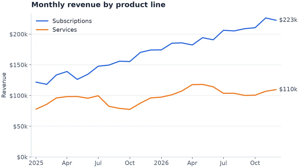

A matplotlib line chart of monthly revenue by product line over 24 months: Subscriptions rising to $223k and Services to $110k, with the last values labelled

Example 1. Invented data.

2. Bar chart with value labels

ax.bar_label puts each value above its bar in one line. Leave headroom with set_ylim so the tallest label isn't clipped.

# Invented data: orders by region last quarter
regions = ["North", "South", "East", "West", "Central"]
orders = [1840, 1325, 2210, 1960, 980]
 
fig, ax = plt.subplots(figsize=(8, 4.5), layout="constrained")
bars = ax.bar(regions, orders, width=0.55, color=COLORS[0])
ax.bar_label(bars, labels=[f"{v:,}" for v in orders], padding=4, color="#334155")
 
ax.set_title("Orders by region, Q3")
ax.set_ylabel("Orders")
ax.yaxis.set_major_formatter("{x:,.0f}")
ax.set_ylim(0, max(orders) * 1.12)  # headroom so the top label is not clipped
ax.tick_params(axis="x", length=0)
 
fig.savefig("orders-by-region.png", dpi=200)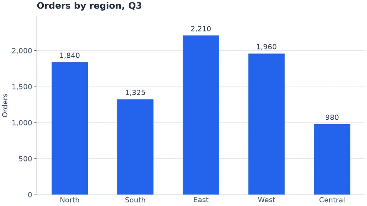

A matplotlib bar chart of orders by region in Q3, with North 1,840, South 1,325, East 2,210, West 1,960 and Central 980 labelled above the bars

Example 2. Invented data.

3. Sorted horizontal bar chart

With more than five or six categories, or long names, turn the bars sideways and sort them so the largest is on top.

# Invented data: revenue by product, year to date (USD thousands)
products = ["Starter plan", "Team plan", "Business plan", "Enterprise plan", "Onboarding",
            "Training", "Support add-on", "API credits", "Storage add-on", "Consulting"]
revenue = np.array([310, 545, 720, 980, 120, 95, 210, 265, 140, 405])
 
order = np.argsort(revenue)  # ascending, so the largest ends up at the top
fig, ax = plt.subplots(figsize=(8, 4.5), layout="constrained")
bars = ax.barh(np.array(products)[order], revenue[order], height=0.6, color=COLORS[0])
ax.bar_label(bars, labels=[f"${v:,}k" for v in revenue[order]], padding=4, color="#334155")
 
ax.set_title("Revenue by product, year to date")
ax.grid(axis="y", visible=False)
ax.grid(axis="x", visible=True)
ax.xaxis.set_major_formatter("${x:,.0f}k")
ax.set_xlim(0, revenue.max() * 1.12)
ax.tick_params(axis="y", length=0)
 
fig.savefig("revenue-by-product.png", dpi=200)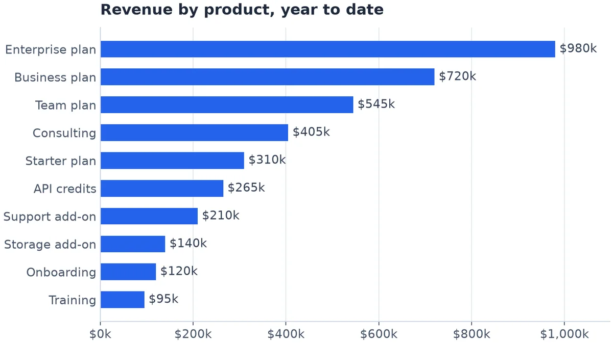

A matplotlib horizontal bar chart of revenue by product year to date, sorted from Enterprise plan at $980k down to Training at $95k

Example 3. Invented data.

4. Stacked bar chart with totals

Revenue by channel each quarter, with the total written above each stack. A thin white edge separates the segments.

# Invented data: quarterly revenue by sales channel (USD thousands)
quarters = ["Q1", "Q2", "Q3", "Q4"]
channels = {
    "Online": np.array([420, 465, 510, 590]),
    "Retail": np.array([310, 295, 320, 380]),
    "Partners": np.array([150, 185, 210, 240]),
}
 
fig, ax = plt.subplots(figsize=(8, 4.5), layout="constrained")
bottom = np.zeros(len(quarters))
for (name, values), color in zip(channels.items(), COLORS):
    ax.bar(quarters, values, bottom=bottom, width=0.55, label=name, color=color,
           edgecolor="white", linewidth=1.5)  # thin white gap between segments
    bottom += values
 
# Total on top of each stack
for x, total in enumerate(bottom):
    ax.text(x, total + 15, f"${total:,.0f}k", ha="center", va="bottom", color="#334155")
 
ax.set_title("Quarterly revenue by channel")
ax.set_ylabel("Revenue")
ax.yaxis.set_major_formatter("${x:,.0f}k")
ax.set_ylim(0, bottom.max() * 1.12)
ax.tick_params(axis="x", length=0)
ax.legend(ncols=3, loc="upper left")
 
fig.savefig("revenue-by-channel.png", dpi=200)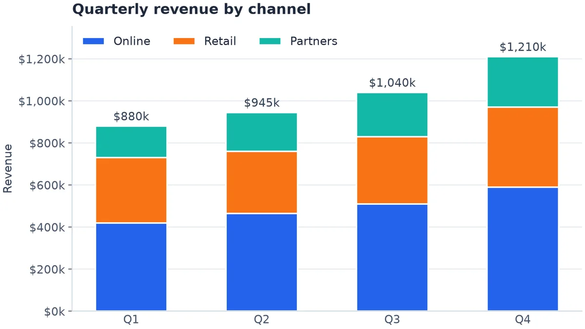

A matplotlib stacked bar chart of quarterly revenue by channel, Online, Retail and Partners, with totals of $880k, $945k, $1,040k and $1,210k above the bars

Example 4. Invented data.

5. Histogram with a median line

Order values are usually skewed: many small orders, a few large ones. A histogram shows the shape, and the median is a better "typical order" than the average.

# Invented data: value of 5,000 orders (USD), right-skewed like most order values
rng = np.random.default_rng(7)
order_values = rng.lognormal(mean=4.0, sigma=0.55, size=5000)
median = np.median(order_values)
 
fig, ax = plt.subplots(figsize=(8, 4.5), layout="constrained")
ax.hist(order_values, bins=np.arange(0, 260, 10), color=COLORS[0], edgecolor="white", linewidth=1)
ax.axvline(median, color="#1E293B", linewidth=1.5, linestyle="--")
ax.annotate(f"Median ${median:,.0f}", xy=(median, 0.97), xycoords=("data", "axes fraction"),
            xytext=(6, 0), textcoords="offset points", va="top", color="#1E293B")
 
ax.set_title("Distribution of order values")
ax.set_xlabel("Order value (USD)")
ax.set_ylabel("Number of orders")
ax.xaxis.set_major_formatter("${x:,.0f}")
ax.set_xlim(0, 250)
 
fig.savefig("order-values.png", dpi=200)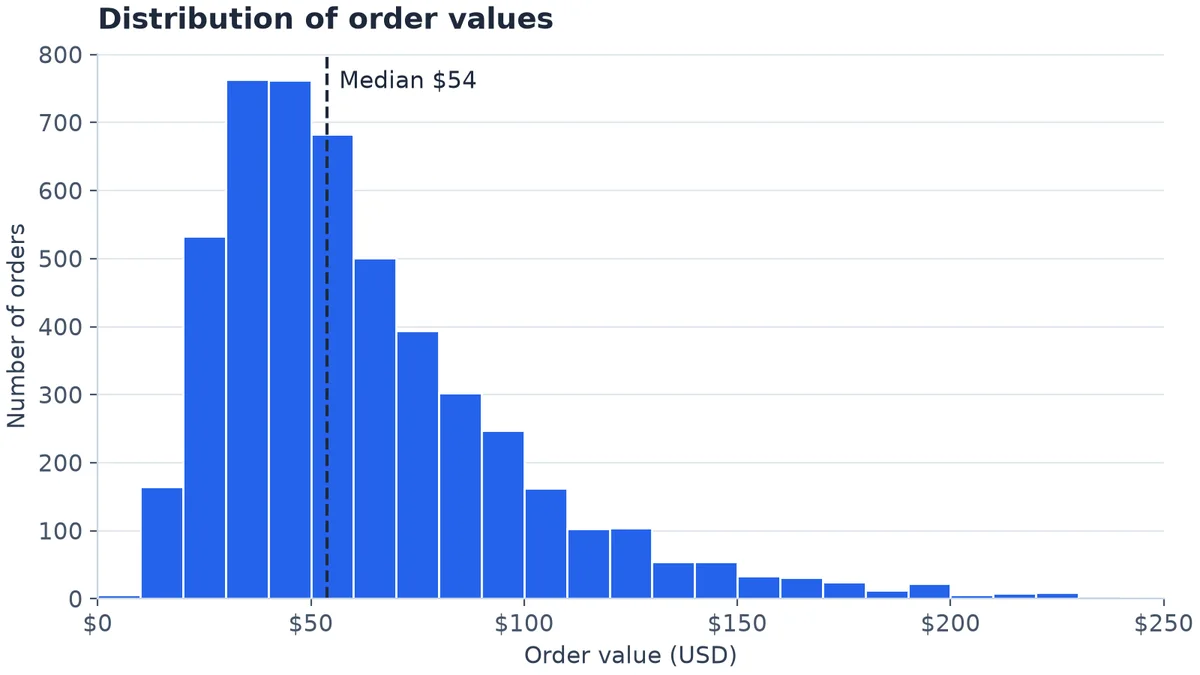

A matplotlib histogram of 5,000 order values in $10 bins, peaking around $40 with a long tail to $250, and a dashed line marking the median at $54

Example 5. Invented data.

6. Scatter plot coloured by category

Ad spend against revenue for campaigns in three channels. One scatter call per group gives each its colour and a legend entry; a white edge keeps overlapping points apart.

# Invented data: monthly ad spend vs. revenue for 60 campaigns in three channels
rng = np.random.default_rng(3)
channels = {"Search": (2.6, 6), "Social": (1.8, 7), "Email": (4.0, 3)}  # (return per $1, max spend)
 
fig, ax = plt.subplots(figsize=(8, 4.5), layout="constrained")
for (name, (ratio, max_spend)), color in zip(channels.items(), COLORS):
    spend = rng.uniform(1, max_spend, 20)                   # USD thousands
    revenue = spend * ratio * rng.normal(1, 0.18, 20)       # USD thousands
    ax.scatter(spend, revenue, s=45, color=color, label=name,
               edgecolor="white", linewidth=0.8, alpha=0.9)
 
ax.set_title("Ad spend vs. revenue by channel")
ax.set_xlabel("Monthly ad spend")
ax.set_ylabel("Attributed revenue")
ax.grid(axis="x", visible=True)
ax.xaxis.set_major_formatter("${x:,.0f}k")
ax.yaxis.set_major_formatter("${x:,.0f}k")
ax.set_xlim(0, None)
ax.set_ylim(0, None)
ax.legend(title="Channel", loc="upper left", alignment="left")
 
fig.savefig("spend-vs-revenue.png", dpi=200)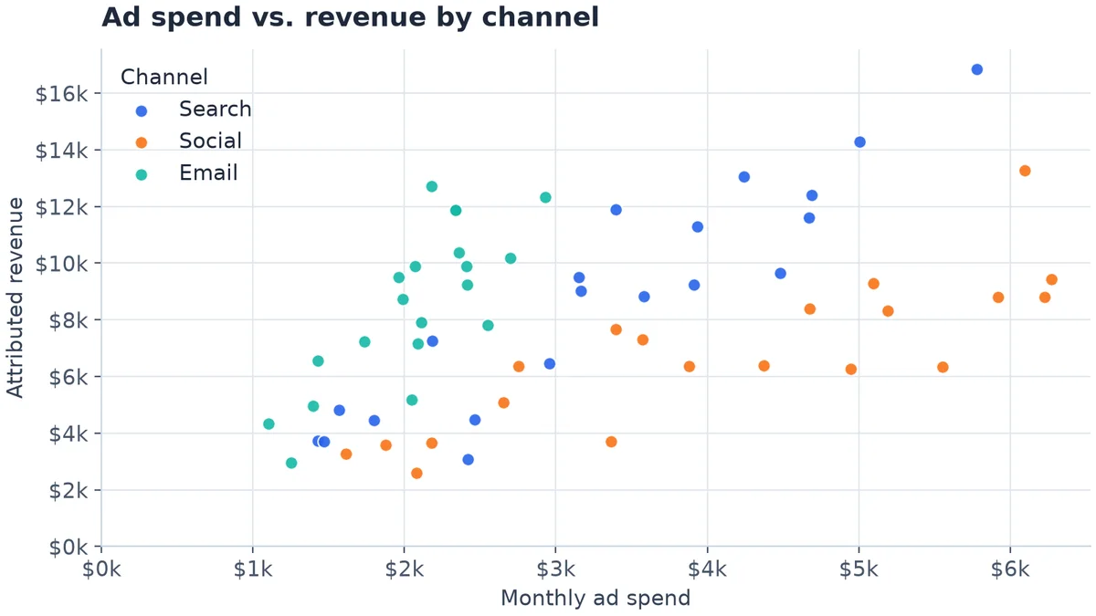

A matplotlib scatter plot of monthly ad spend against attributed revenue for 60 campaigns, coloured by channel: Search, Social and Email

Example 6. Invented data.

Jupyter notebooks for your team.

Start free →

7. A one-page KPI grid with subplots

Four charts on one figure for a weekly summary. plt.subplots(2, 2) returns a grid of axes; fill each one, and fig.suptitle titles the page.

# Invented data for a one-page KPI summary
rng = np.random.default_rng(11)
months = ["Jan", "Feb", "Mar", "Apr", "May", "Jun", "Jul", "Aug", "Sep", "Oct", "Nov", "Dec"]
revenue = 200 + np.cumsum(rng.normal(8, 10, 12))            # USD thousands
regions = ["North", "South", "East", "West"]
orders = [1840, 1325, 2210, 1960]
order_values = rng.lognormal(4.0, 0.5, 2000)                # USD
conversion = 2.1 + np.cumsum(rng.normal(0.05, 0.12, 12))    # percent
 
fig, axs = plt.subplots(2, 2, figsize=(8, 6), layout="constrained")
fig.suptitle("Sales overview, 2026", x=0.02, ha="left", fontsize=15, fontweight="bold")
 
ax = axs[0, 0]
ax.plot(months, revenue, linewidth=2, color=COLORS[0])
ax.set_title("Monthly revenue", fontsize=12)
ax.yaxis.set_major_formatter("${x:,.0f}k")
ax.set_xticks(months[::3])
 
ax = axs[0, 1]
ax.bar(regions, orders, width=0.55, color=COLORS[0])
ax.set_title("Orders by region", fontsize=12)
ax.yaxis.set_major_formatter("{x:,.0f}")
ax.tick_params(axis="x", length=0)
 
ax = axs[1, 0]
ax.hist(order_values, bins=np.arange(0, 260, 10), color=COLORS[0], edgecolor="white", linewidth=0.8)
ax.set_title("Order value distribution", fontsize=12)
ax.set_xlim(0, 250)
ax.xaxis.set_major_formatter("${x:,.0f}")
 
ax = axs[1, 1]
ax.plot(months, conversion, linewidth=2, color=COLORS[0])
ax.set_title("Conversion rate", fontsize=12)
ax.yaxis.set_major_formatter("{x:.1f}%")
ax.set_xticks(months[::3])
 
fig.savefig("kpi-grid.png", dpi=200)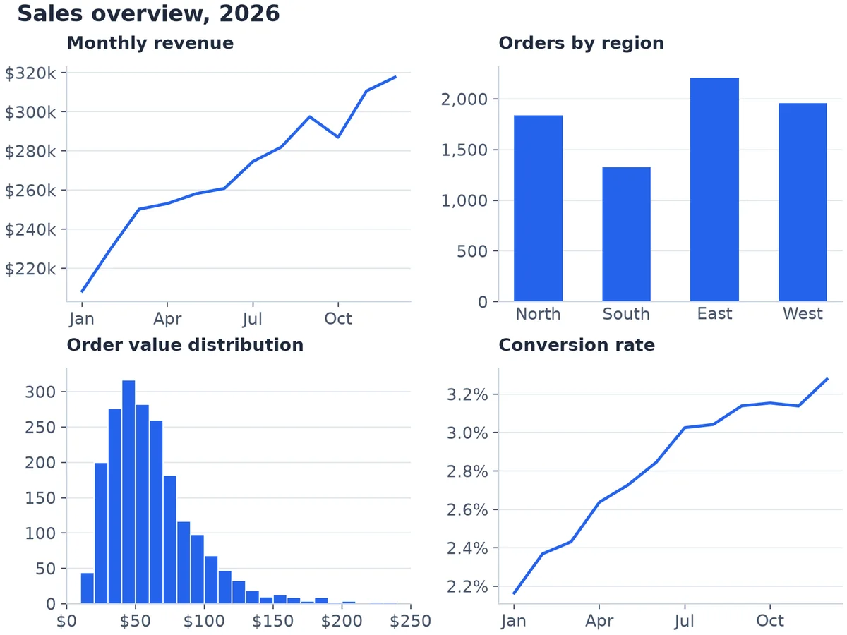

A matplotlib 2-by-2 grid titled Sales overview, 2026: monthly revenue line, orders by region bars, order value histogram and conversion rate line

Example 7. Invented data.

8. Small multiples instead of a second y-axis

When you want to compare many series, or two measures on different scales, don't add a second y-axis: readers misjudge which line belongs to which scale. Draw one small chart per series with shared axes, each highlighting its own line over the others in grey.

# Invented data: weekly sales for six regions over one year (USD thousands)
rng = np.random.default_rng(5)
weeks = np.arange(1, 53)
regions = ["North", "South", "East", "West", "Central", "Online"]
sales = {r: 40 + 4 * i + np.cumsum(rng.normal(0.3, 2.2, 52)) for i, r in enumerate(regions)}
 
fig, axs = plt.subplots(2, 3, figsize=(8, 5), sharex=True, sharey=True, layout="constrained")
fig.suptitle("Weekly sales by region (USD thousands)", x=0.02, ha="left", fontsize=15, fontweight="bold")
for ax, region in zip(axs.flat, regions):
    for other in regions:  # every region in light gray, for context
        ax.plot(weeks, sales[other], color="#CBD5E1", linewidth=1)
    ax.plot(weeks, sales[region], color=COLORS[0], linewidth=2)  # this panel's region on top
    ax.set_title(region, fontsize=12)
    ax.set_xticks([1, 13, 26, 39, 52])
for ax in axs[1]:
    ax.set_xlabel("Week")
 
fig.savefig("sales-by-region.png", dpi=200)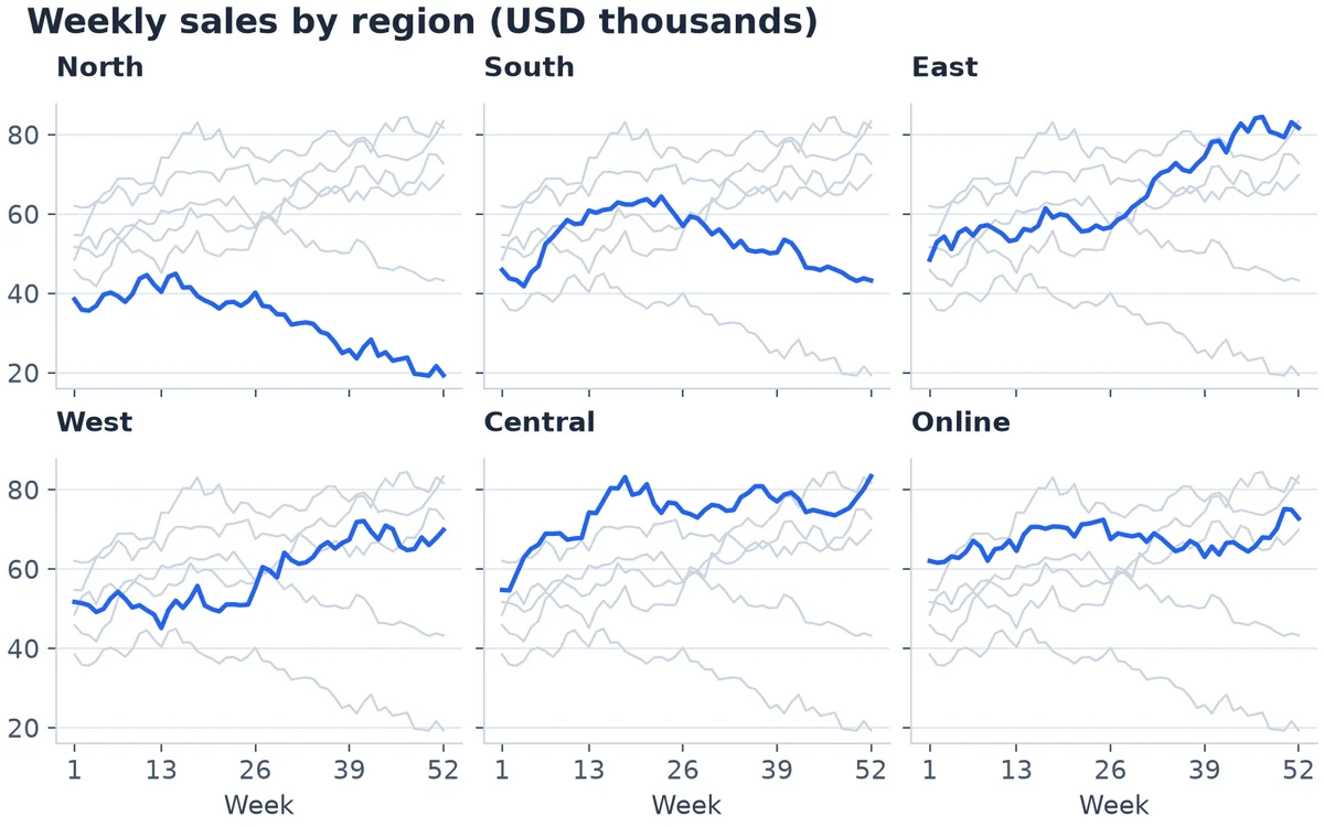

Six matplotlib small multiples of weekly sales by region, each panel highlighting one region in blue over the others in grey: North, South, East, West, Central and Online

Example 8. Invented data.

9. Daily data with a 7-day rolling average

Daily numbers are noisy: weekends dip, one-off days spike. Plot the raw line thin and grey and a 7-day average on top, and shade events such as a promotion with axvspan. This one uses pandas for the rolling average.

import matplotlib.dates as mdates
import pandas as pd
 
# Invented data: daily orders for 120 days, with a weekly rhythm and a promotion
rng = np.random.default_rng(21)
days = pd.date_range("2026-06-01", periods=120, freq="D")
weekly = np.where(days.dayofweek >= 5, -25, 10)             # quieter weekends
promo = (days >= "2026-08-10") & (days <= "2026-08-23")
orders = 320 + np.arange(120) * 0.6 + weekly + promo * 90 + rng.normal(0, 18, 120)
df = pd.DataFrame({"orders": orders.round()}, index=days)
df["avg_7d"] = df["orders"].rolling(7).mean()
 
fig, ax = plt.subplots(figsize=(8, 4.5), layout="constrained")
ax.axvspan(pd.Timestamp("2026-08-10"), pd.Timestamp("2026-08-23"), color="#F1F5F9")
ax.text(pd.Timestamp("2026-08-16 12:00"), 525, "Summer promo", ha="center", color="#475569")
ax.plot(df.index, df["orders"], color="#94A3B8", linewidth=1, label="Daily orders")
ax.plot(df.index, df["avg_7d"], color=COLORS[0], linewidth=2.2, label="7-day average")
 
ax.set_title("Daily orders with 7-day average")
ax.set_ylabel("Orders per day")
ax.xaxis.set_major_locator(mdates.MonthLocator())
ax.xaxis.set_major_formatter(mdates.ConciseDateFormatter(ax.xaxis.get_major_locator()))
ax.set_ylim(200, 545)
ax.legend(loc="upper left", ncols=2)
 
fig.savefig("daily-orders.png", dpi=200)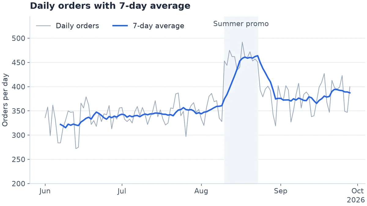

A matplotlib line chart of daily orders from June to September 2026, with the noisy daily line in grey, a 7-day average in blue, and a shaded summer promotion in August

Example 9. Invented data.

10. Heatmap: weekday by hour

When orders come in, by day of week and hour. imshow draws the grid, a single-colour scale from light to dark shows the amount, and a colour bar explains it.

# Invented data: average orders by weekday and hour of day
rng = np.random.default_rng(9)
weekdays = ["Mon", "Tue", "Wed", "Thu", "Fri", "Sat", "Sun"]
hours = np.arange(24)
daily_shape = np.exp(-((hours - 13) ** 2) / 18) + 0.6 * np.exp(-((hours - 20) ** 2) / 6)
day_level = np.array([1.0, 1.05, 1.1, 1.08, 0.95, 0.7, 0.6])
orders = (np.outer(day_level, daily_shape) * 60 + rng.normal(0, 2, (7, 24))).clip(min=0)
 
fig, ax = plt.subplots(figsize=(8, 4.5), layout="constrained")
im = ax.imshow(orders, cmap="Blues", aspect="auto")
ax.set_xticks(hours[::3], labels=[f"{h:02d}:00" for h in hours[::3]])
ax.set_yticks(range(len(weekdays)), labels=weekdays)
ax.grid(False)
ax.tick_params(length=0)
for spine in ax.spines.values():
    spine.set_visible(False)
cbar = fig.colorbar(im, ax=ax, shrink=0.85)
cbar.set_label("Average orders per hour")
cbar.outline.set_visible(False)
ax.set_title("When orders come in: weekday by hour")
 
fig.savefig("orders-heatmap.png", dpi=200)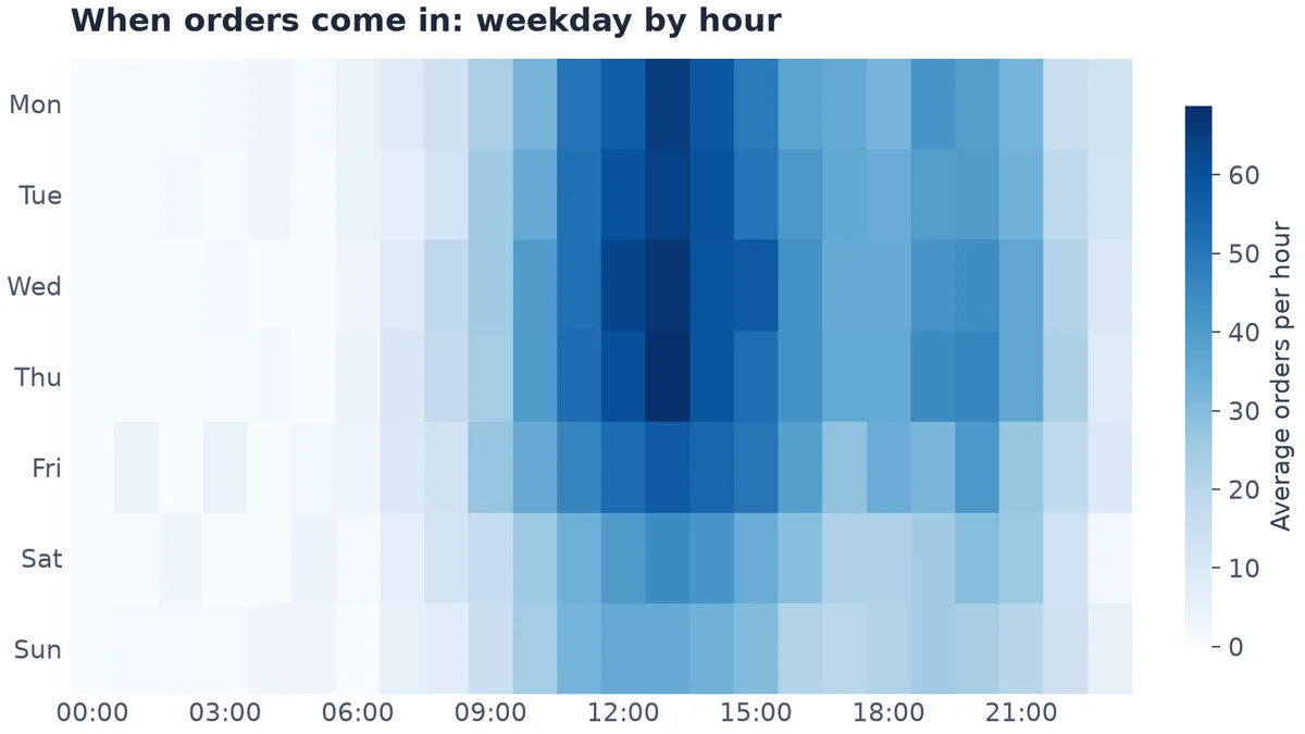

A matplotlib heatmap of average orders per hour by weekday, darkest around midday on weekdays with a smaller evening peak and lighter weekends

Example 10. Invented data.

Pyplot or the object-oriented style?

Every example above uses the object-oriented style: create a figure and axes with plt.subplots, then call methods on ax. Matplotlib's own guidance: "In general, we suggest using the OO style, particularly for complicated plots, and functions and scripts that are intended to be reused as part of a larger project. However, the pyplot style can be very convenient for quick interactive work." plt.plot(x, y) is fine for a quick look; switch to fig, ax = plt.subplots() as soon as a chart has more than one part.

For hundreds more examples, matplotlib's official gallery covers every chart type and lets you download them all, as Python files or as Jupyter notebooks.

Run them on your real data

These examples generate their own numbers. To chart your own, replace the invented data with a query result. In a Fastero notebook, a SQL cell runs on one of your workspace's databases and hands the rows to Python as a pandas DataFrame, so the next cell can draw any of these charts from live numbers. The notebook can then run on a schedule, and a cell's result can be pinned to a dashboard your team opens.

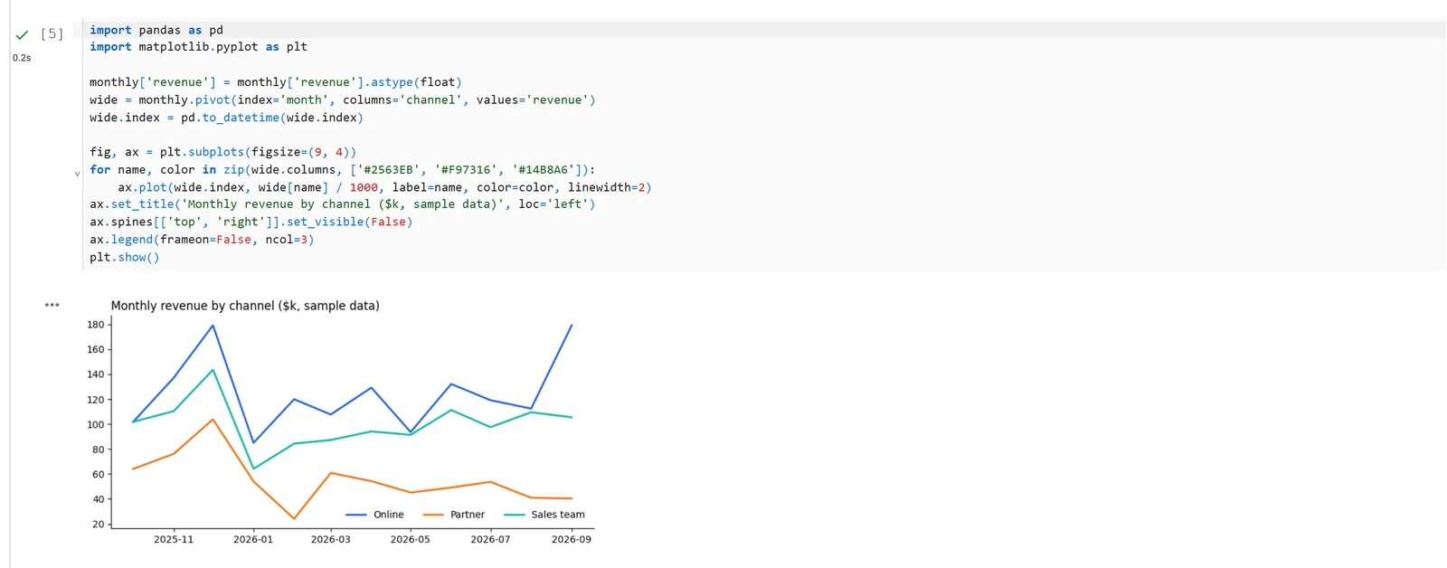
A Fastero notebook cell: Python that pivots monthly revenue by channel and plots it with matplotlib, above a line chart of Online, Partner and Sales team revenue

A matplotlib chart in a Fastero notebook, drawn from the DataFrame a SQL cell returned. Sample data.

FAQ

What is the latest version of matplotlib?

Matplotlib 3.11.2, released in September 2026. It needs Python 3.11 or later. We also ran two of the examples above in a Fastero notebook on matplotlib 3.10.3, unchanged.

Where is the official matplotlib gallery?

At matplotlib.org/stable/gallery. Every example has its source code, and the whole gallery can be downloaded as Python files or as Jupyter notebooks.

How do I add value labels to a bar chart in matplotlib?

Use ax.bar_label(bars), where bars is what ax.bar or ax.barh returned. Pass labels= to format them and padding= to move them off the bar, as in examples 2 and 3.

How do I stop matplotlib cutting off labels?

Create the figure with plt.subplots(..., layout="constrained"), which makes room for titles, labels and legends. For labels above bars, also raise the axis limit with ax.set_ylim(0, max_value * 1.12).

How do I format dates on a matplotlib axis?

Set a locator, such as mdates.MonthLocator(), and mdates.ConciseDateFormatter for the labels. It shows the year once instead of on every tick, as in examples 1 and 9.

How do I save a high-resolution matplotlib chart?

fig.savefig("chart.png", dpi=200). An 8-inch-wide figure at 200 dpi gives a 1,600-pixel image, sharp on most screens and slides.

Related reading:

Sources: Matplotlib gallery, Matplotlib quick start, ConciseDateFormatter example, matplotlib on PyPI. All ten examples run on 5 November 2026 with matplotlib 3.11.2, NumPy 2.5.4 and pandas 2.3.3 on Python 3.14.3.

Try Fastero free — run these charts on your own database in a hosted notebook, on a schedule, and share them with free viewers. No credit card required.