 Fastero Dev Team
Bar charts and histograms both draw rectangles, which is why they get mixed up. They answer different questions, and the quickest way to see the difference is to draw both from the same data. Every chart below comes from one file of 4,734 invented orders.
The short answer: a bar chart compares a number across separate categories, such as revenue by product category. Each bar is one category, the bars have gaps between them, and you can sort them in any order. A histogram shows how the values of one number are spread out, such as the value of each order. It cuts the number line into ranges called bins and counts the values in each, so the bars touch, stay in numeric order, and change shape when you change the bin width. Use a bar chart to compare groups. Use a histogram to see what's typical, how wide the spread is, and where the gaps are.
Fastero
Connect your database. Ask questions. Get dashboards.
Postgres, BigQuery, Snowflake, and 10+ sources — live-connected, AI-powered, no dashboard builder learning curve.
Try free →Bar chart vs histogram at a glance
| Bar chart | Histogram | |
|---|---|---|
| Answers | How do these categories compare? | How are the values of one number spread out? |
| Horizontal axis | Categories (names) | A number, cut into bins |
| Bar height | Any measure: a sum, an average, a count | How many values fall in the bin |
| Gaps between bars | Yes | No: a gap means an empty bin |
| Order of bars | Your choice, usually largest first | Fixed: low to high |
| What changes the picture | Which measure you choose | The bin width |
| The SQL behind it | GROUP BY category |
GROUP BY floor(value / width) |
The data
sample-sales.csv holds 4,734 invented orders from 1 November 2024 to 31 October 2026, one row per order, with a category, a product and the order's revenue. It's the sample every new Fastero workspace starts with. We ran the queries in DuckDB 2.0.0 and drew the charts with matplotlib 3.11.2 on Python 3.14.3, on 18 November 2026. This is the core of the script, without the styling:
import numpy as np
import pandas as pd
import matplotlib.pyplot as plt

sales = pd.read_csv("sample-sales.csv")

# Bar chart: sum revenue per category, sort, one bar each
by_category = sales.groupby("category")["revenue"].sum().sort_values(ascending=False)
fig, ax = plt.subplots(figsize=(8, 4.5), layout="constrained")
ax.bar(by_category.index, by_category.values, width=0.6)

# Histogram: the value of every order, counted in $50 bins
fig, ax = plt.subplots(figsize=(8, 4.5), layout="constrained")
ax.hist(sales["revenue"], bins=np.arange(0, 1900, 50), edgecolor="white")
The bar chart: revenue by category
A bar chart adds up a measure per category. In SQL that's a GROUP BY on a column that already exists:
select category, round(sum(revenue)) as revenue
from sales
group by category
order by revenue desc;
┌──────────┬──────────┐
│ category │ revenue │
│ varchar │ double │
├──────────┼──────────┤
│ Hardware │ 704343.0 │
│ Software │ 374298.0 │
│ Supplies │ 198372.0 │
│ Services │ 196687.0 │
└──────────┴──────────┘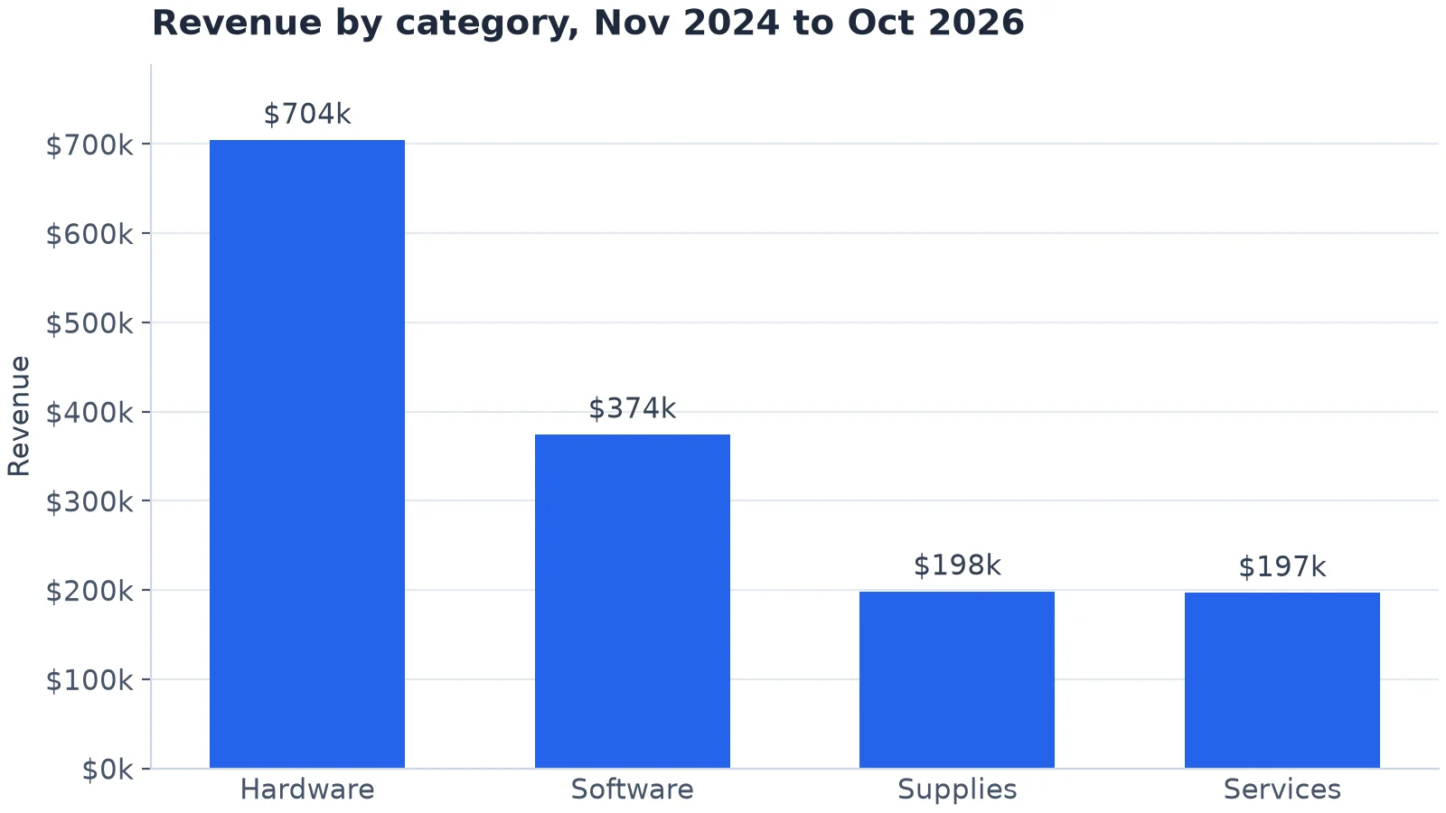
A bar chart: one bar per category, sorted by size. Invented data.
The order of the bars is yours to choose, and largest first is easiest to read. The measure is yours to choose too: Supplies has the most orders (1,628) but ranks third on revenue, so a bar chart of order counts would put it first.
The histogram: what does an order look like?
A histogram uses one numeric column without adding it up: here, the revenue of each of the 4,734 orders. Matplotlib's hist cuts the range into $50 bins and counts the orders in each.
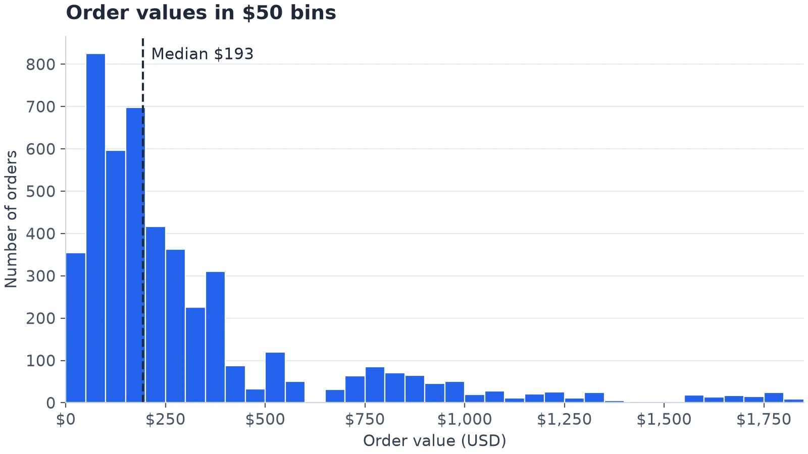
The same orders as a histogram, in $50 bins. The bars touch; the two gaps are real. Invented data.
A typical order is small: the median is $193, while the mean is $311, pulled up by a long tail of large orders. There's a second group of orders between about $700 and $1,000. And there are two empty stretches: no order is worth between $581.64 and $665.48, or between $1,358.64 and $1,551.56.
Bin width changes the story
Here are the same 4,734 orders in $500 bins.
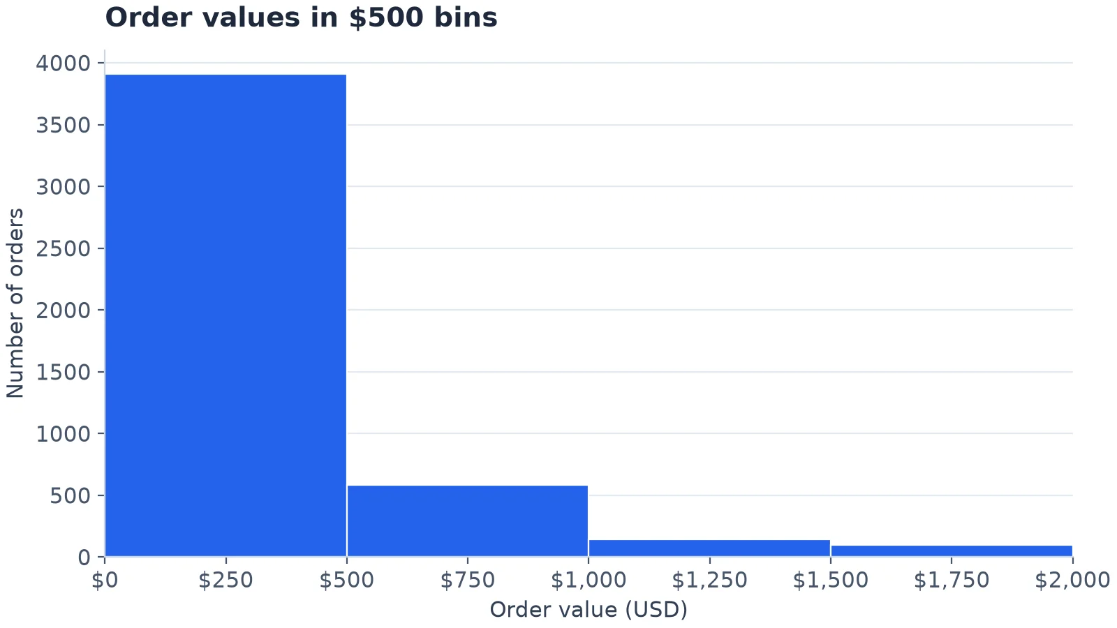
The same orders in $500 bins: the second group and both gaps disappear. Invented data.
Four bars: 3,909 orders under $500, then 584, 144 and 97. The story is now that most orders are small and a few are big. That's true, but the second group and both gaps are gone. Neither chart is wrong; the wide one answers a coarser question. So try two or three widths before you settle, and put the width in the axis label.
If you don't choose, your tool does:
| Rule | What it picked for these 4,734 orders |
|---|---|
| Matplotlib's default | 10 bins, each $180 wide |
NumPy bins="sturges" |
14 bins of $128.57 |
NumPy bins="auto" (also "fd" here) |
59 bins of $30.51 |
| Our choice | 37 bins of $50 |
NumPy's "auto" takes the "Minimum bin width between the 'sturges' and 'fd' estimators" and, NumPy's docs say, for larger datasets "will usually default to FD", which is what happened here. Treat the automatic result as a first look, then round the width to something a reader can say out loud, like $50.
Connect any database. Ask in plain English.
Start free →Three mistakes that make a histogram lie
1. Gaps between bars, or no gaps where there should be
A histogram's bars touch, so a visible gap means an empty bin. The trap is building one in SQL: GROUP BY returns only bins that have rows, so the empty $600 to $650 bin vanishes from the result.
select floor(revenue / 50) * 50 as bin_start, count(*) as orders
from sales
where revenue >= 500 and revenue < 750
group by bin_start
order by bin_start;
┌───────────┬────────┐
│ bin_start │ orders │
│ double │ int64 │
├───────────┼────────┤
│ 500.0 │ 120 │
│ 550.0 │ 50 │
│ 650.0 │ 32 │
│ 700.0 │ 64 │
└───────────┴────────┘Chart those four rows as categories and the gap closes. Generate every bin first and left-join the data to it, so empty bins come back as zero:
with bins as (
  select range as bin_start from range(500, 750, 50)
)
select bin_start, count(s.order_id) as orders
from bins
left join sales s on s.revenue >= bin_start and s.revenue < bin_start + 50
group by bin_start
order by bin_start;
┌───────────┬────────┐
│ bin_start │ orders │
│ int64 │ int64 │
├───────────┼────────┤
│ 500 │ 120 │
│ 550 │ 50 │
│ 600 │ 0 │
│ 650 │ 32 │
│ 700 │ 64 │
└───────────┴────────┘2. Sorting a histogram by height
The horizontal axis of a histogram is a number line. Sort the bars from tallest to shortest and the $50 to $100 bin lands next to the $150 to $200 bin, and the shape you were trying to see is gone. Sorting is right for a bar chart of categories and wrong for a histogram.
3. Unequal bins drawn as counts
Bins don't have to be the same width, but then a bar's height can't be a plain count. With bins of $0 to $100, $100 to $200, $200 to $500 and $500 to $2,000, the counts are 1,179, 1,294, 1,436 and 825. Drawn as bars, the last bin looks more than half as busy as the others, though it covers 15 times the range. Divide each count by its width and the picture is honest: 1,179, 1,294, 479 and 55 orders per $100 of order value.
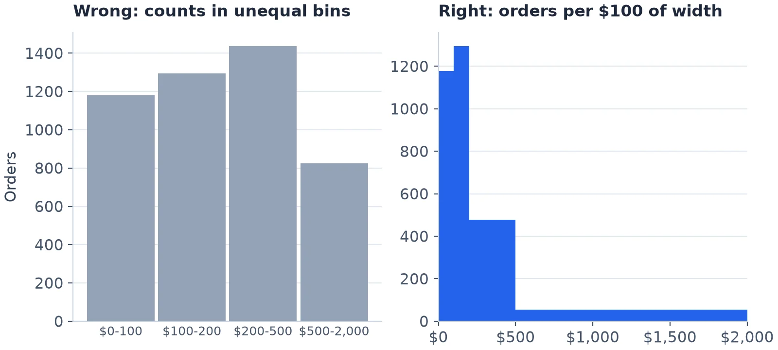
Unequal bins: plain counts on the left, counts per $100 of width on the right. Invented data.
In matplotlib, density=True does the division for you: its docs define it as "density = counts / (sum(counts) * np.diff(bins))", so the bars' areas add up to 1.
One mistake belongs to bar charts: an axis that doesn't start at zero. A bar's length is its value, so starting the axis at $150k would make Hardware's bar about 12 times as tall as Services' rather than about 3.6 times.
When to use which
- A bar chart when the question is about categories: revenue by category, orders by channel, sign-ups by plan. It's also fine for a count of a few whole numbers, such as orders by quantity, where each value is its own category.
- A histogram when the question is about one continuous number: order values, delivery times, response times, ages. Draw one before you quote an average. If it's lopsided, as these order values are, quote the median.
- A box plot or one histogram per category when you want both: how order values differ between categories. Our guide to types of charts has a box plot of exactly that.
When the chart has to stay current
The charts above are pictures of one file. At work, the same bar chart is usually wanted every Monday, on the latest orders, where colleagues can open it.
Fastero is an AI and data platform where people and AI agents work together on a team's data. For charts that means:
- A chart is a saved SQL query on a connected database or warehouse, not a copy of the data. Ask for one in plain English and the AI agent writes the SQL and draws the chart; the query stays with it so you can check every number.
- Refresh: a dashboard refreshes on a timer (1, 5, 15 or 60 minutes) or, for Postgres and BigQuery data only, when the data changes.
- Files: a chart from an uploaded CSV or Excel file is a snapshot of that file. To update it, upload the file again.
- Sharing: colleagues sign in to see it and viewers are free, or it goes out by scheduled email with a PDF.
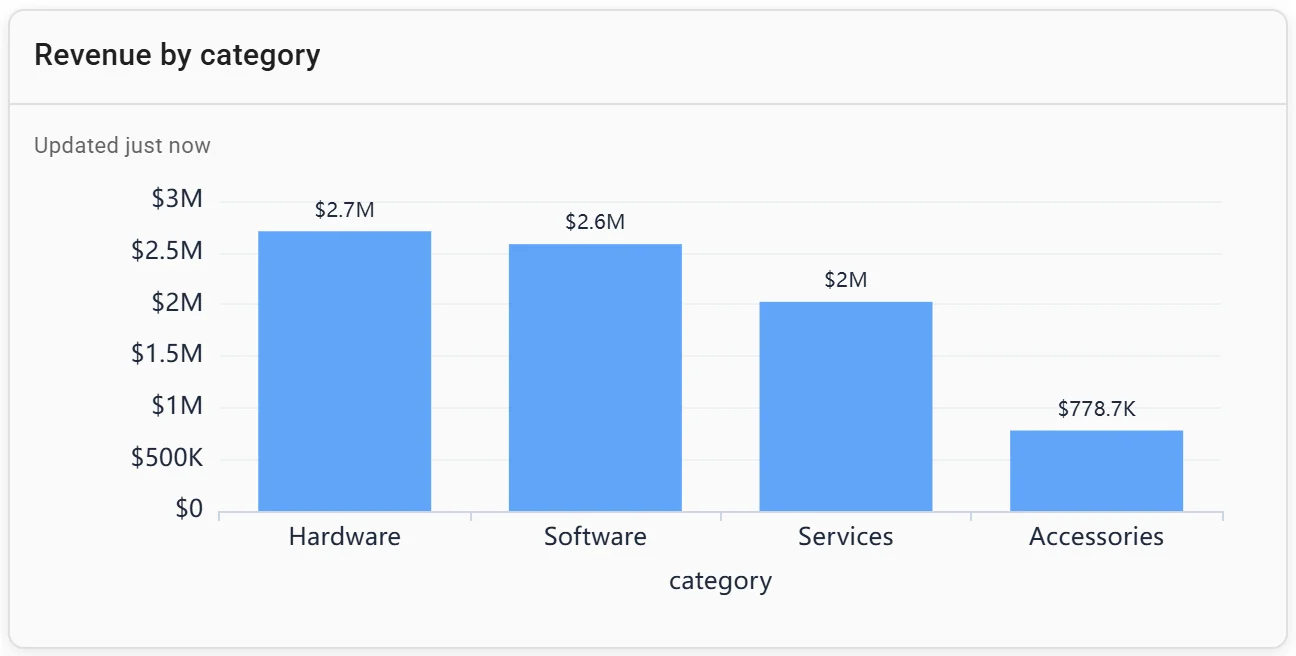
A bar chart: revenue by category. Invented data.
More on making a chart from a SQL query, matplotlib examples and AI chart generators.
FAQ
What is the main difference between a bar chart and a histogram?
A bar chart compares a measure across categories, such as revenue by product category. A histogram shows the distribution of one numeric variable by counting how many values fall in each range, such as how many orders are worth $50 to $100.
Why do the bars in a histogram touch?
Because the bins are next to each other on a number line: one ends where the next begins. A gap between histogram bars should mean a bin with no values in it.
Can a histogram have gaps?
Yes, when a bin is empty. In our sample, no order is worth between $581.64 and $665.48, so the $600 to $650 bin has no bar. If you build the histogram in SQL, make sure empty bins come back as zero, or the gap disappears.
How many bins should a histogram have?
There's no single right number. Start with your tool's automatic choice, such as NumPy's bins="auto", then try two or three round widths and keep the one that shows the shape without turning to noise. On 4,734 order values, "auto" picked 59 bins and $50 bins gave 37.
Is a histogram a type of bar chart?
It's drawn with bars, but it works differently. A bar chart's bars are categories, in any order, measured any way you like; a histogram's bars are ranges of one number, in fixed order, and their heights are counts.
Sources
Read on 18 November 2026:
- NumPy: numpy.histogram_bin_edges (the
"auto","fd"and"sturges"rules) - Matplotlib: Axes.hist (default bins,
density) - Data:
sample-sales.csv, 4,734 invented orders. Charts drawn with matplotlib 3.11.2, NumPy 2.5.5 and pandas 3.1.1; SQL run in DuckDB 2.0.0, on Python 3.14.3.